Computer Vision 3
Introduction and Object Detection
What this course is
Hight-level(semantic) computer vision:
-
Object detection
-
image segmentation
-
object tracking
-
etc...
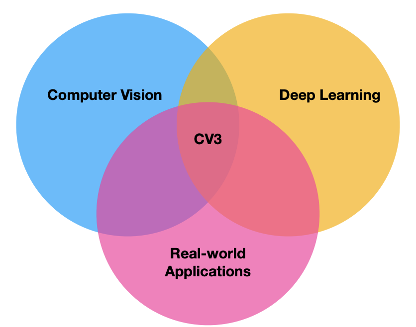
From another perspective this is the intersection of Computer vision, deep learning and real-world applications, as shown in Fig 1.
What is computer vision:
-
First defined in the 60s(The summer vision project 1966).
-
"Mimic the human visual system.
-
Center block of artificial intelligence.
Semantic scene understanding:
-
Classification
-
Object detection
-
Semantic segmentation
-
Instance segmentation
-
Object tracking
This course in two dimension is as shown in Fig 2.
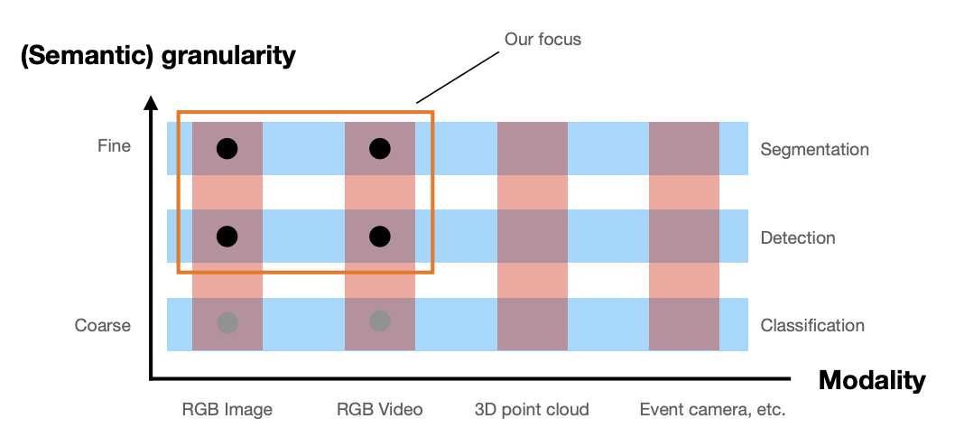
Understanding an image
Different representations depending on the granularity
-
Detection (bounding box-coarse description)
-
Semantic segmentation(pixel-level)
-
Instance segmentation(e.g. "person 1", "person 2")
Understanding a video
Why use the temporal domain
-
Motion analysis, multi-view reasoning.
-
A smoothness assumption: no abrupt changes between frames.
But challenges:
-
High computational demand.
-
A lot of redundancy.
-
Occlusions, multiple objects moving and interacting.
Some architectures and concepts
-
R-CNN, Fast R-CNN and Faster R-CNN (2-stage object detection)
-
YOLO, SSD, RetinaNet (1-stage object detection)
-
Siamese networks (online tracking)
-
Message Passing Networks (offline tracking)
-
Mask R-CNN, UPSNet (panoptic segmentation)
-
Deformable/atrous convolutions
-
Graph neural networks(GNNs)
-
Vision Transformers(ViT), DETR(object detection), SAM
-
Contrastive learning
Object detection
One-stage detectors
One-stage detectors treat object detection as a single task, directly predicting the object class and bounding box coordinates from the input images.
Object detection with sliding window
For every position, measure the distance(or correlation) between the template and the image region(See Fig 3):
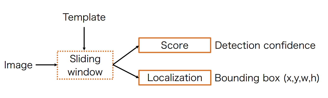
where is the distance metric, is the image
region, and is the template.
Template matching distances
-
Sum of squared distances(SSD), or mean squared error(MSE):
-
Normalized cross-correlation(NCC):
-
Zero-normalized cross-correlation(ZNCC):
Disadvantages
-
(Self-) Occlusions
- e.g. due to pose changes
-
Changes in appearance
-
Unknown position, scale, and aspect ratio
- brute-force search(inefficient)
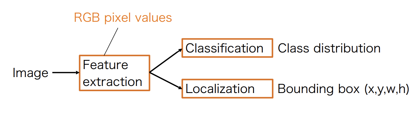
Feature-based detection
Idea: Learn feature-based classifiers invariant to natural object changes(See Fig 4)
-
Features are not always linearly separable
-
Learning multiple weak learners to build a strong classifier(Fig 5)
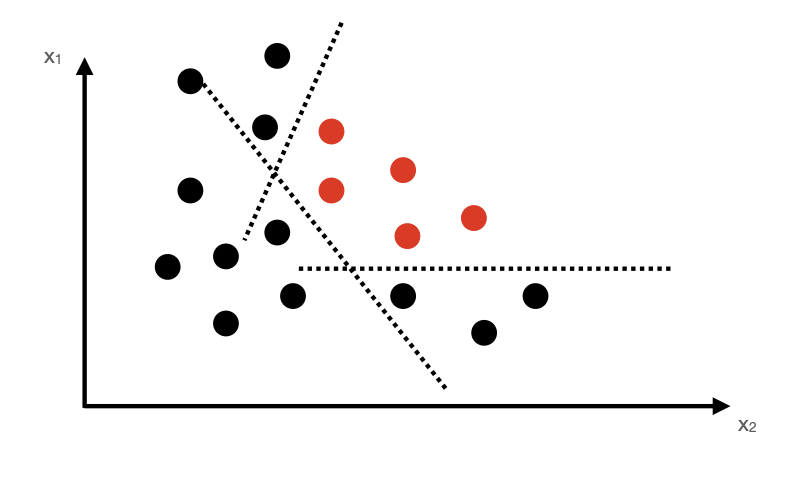
Multiple weak learners
Viola-Jones detector
Given data
-
Define a set of Haar-like features(Fig 6)
Haar-features are sensitive to directionality of patterns
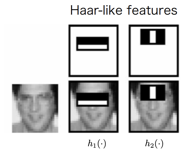
Haar features -
Find a weak classifier with the lowest error across the dataset
-
Save the weak classifier and update the priority of the data samples
-
Repeat Steps 2-3 times
Final classifier is the linear combination of all weak learners.
Histogram of Oriented Gradients
Average gradient image over training samples gradients provide shape information.
HOG descriptor Histogram of oriented gradients.
Compute gradients in dense grids, compute gradients and create a histogram based on gradient direction.
-
Choose your training set of images that contain the object you want to detect.
-
Choose a set of images that do NOT contain that object.
-
Extract HOG features from both sets.
-
Train an SVM classifier on the two sets to detect whether a feature vector represents the object of interest or not(0/1 classification)
Deformable Part Model
Many objects are not rigid, so we could use a Bottom-up approach:
-
detect body parts
-
detect "person" if the body parts are in correct arrangement
Note: The amount of work for each RoI may grow significantly.
Two-stage detectors
Two-stage object detectors split the object detection task to two parts(Fig 7):
-
Region Proposal: The network first identifies potential regions in the image that may contain objects.
-
Refinement: These regions are further analyzed to classify the objects and refine their bounding boxes.
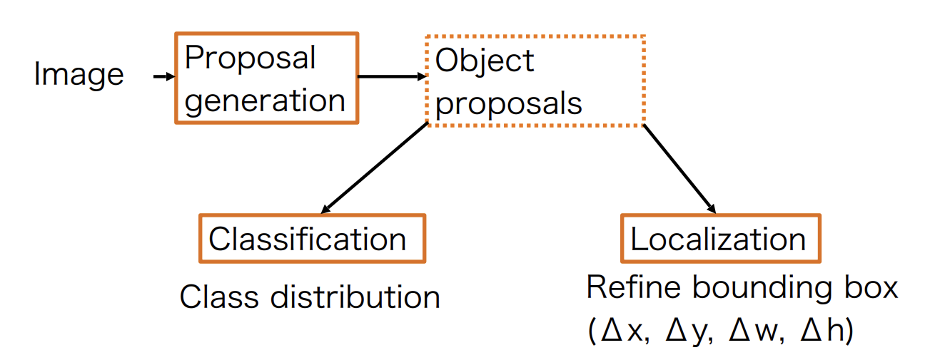
A generic, class-agnostic objectness measure: object proposals or regions of interest(RoI)
Object proposal methods:
-
Selective search
- Using class-agnostic segmentation at multiple scales.
-
Edge boxes
- Bounding boxes that wholly enclose detected contours.
Non-Maximum Suppression(NSM)
Method to keep only the best proposals(See algorithm [alg:nms]).
Region overlap
We measure region overlap with the Intersection over Union(IoU) or Jaccard Index:
The threshold is the decision boundary used to determine whether a detected object or prediction should be considered valid. For example, in object detection:
-
Choosing a high threshold ‒ more false positives, low precision
-
Choosing a low threshold ‒ more false negatives, low recall
Object detection with deep networks
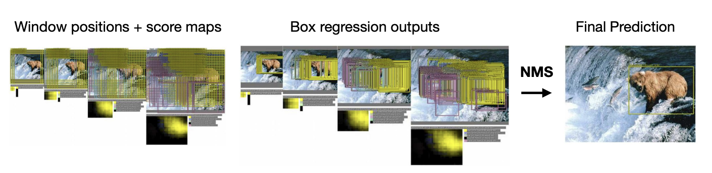
Overfeat
Explores three well-known vision tasks using a single framework.
-
Classification
-
Localization
-
Detection
Training convolution on all tasks boosts up the accuracy, see Fig 8.
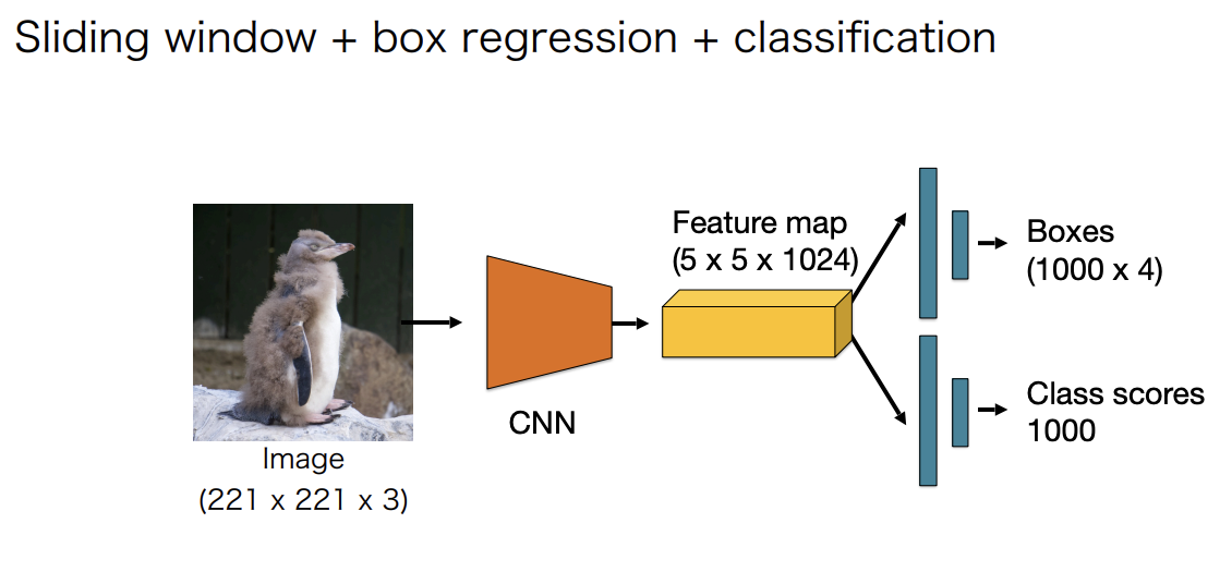
Apply Non-Max Suppression to combine the predictions and windows, see Fig 9.
Improved detection accuracy is largely due to feature representation learned with deep nets.
But cons:
-
Expensive to try all possible positions, scales and aspect ratios.
-
The network operates on a fixed resolution.
The complexity of a sliding window is , where is the number of all the windows, and represents the amount of work needed to perform detection and classification for one window. The complexity of the "pre-filtered" method is , where is the amount of work needed for filtering each window, and is the number of windows left after being filtered.
"Pre-filtering" method pays off when:
Assume the constant factors are comparable/negligible:
where is the Region-of-Interest(RoI) ratio, and is the efficiency of RoI generator. In practice, there is a delicate balance between and : Reducing and increasing .
Object proposals(Pre-filtering) and pooling for two-stage detection
Heuristic-based object proposal methods:
-
Selective search
- Using class-agnostic segmentation at multiple scales.
-
Edge boxes
- Bounding boxes that wholly detected contours
R-CNN family(Regions with CNN features)
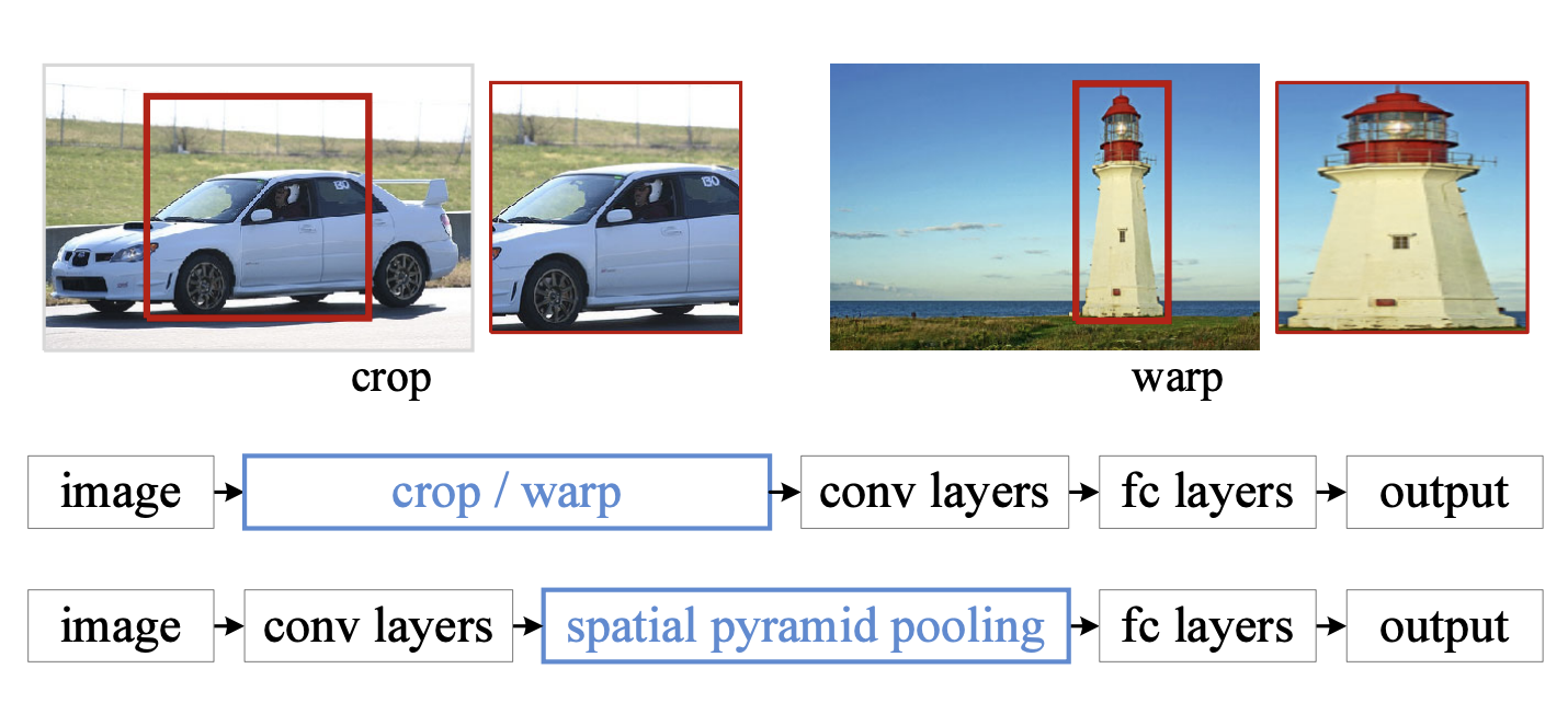
-
Spatial Pyramid Pooling(SPP)
-
(Fast/Faster) R-CNN
-
Region Proposal Network(RPN)
R-CNN
Training scheme:
-
Pre-train the CNN for image classification(ImageNet)
-
Finetune the CNN on the number of classes the detector is aiming to classify
-
Train a linear SVM classifier to classify image regions - one linear SVM per class
-
Train the bounding box regressor
Pros:
-
New: CNN features; the overall pipeline with proposals is heavily engineered – Good accuracy.
-
CNN summarizes each proposal into vector.
-
Leverage transfer learning: The CNN can be pre-trained for image classification with c classes. One needs only to change the FC layers to deal with Z classes.
Cons:
-
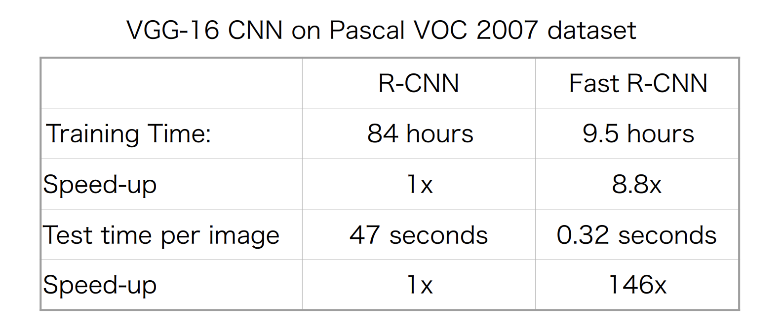
Slow: 47s/image with VGG 16 backbone. One considers around 2000 proposals per image, they need to be warped and forwarded through the CNN.
-
Training is also slow and complex.
-
The object proposal algorithm is fixed.
-
Feature extraction and SVM classifier are trained separately - features are not learned "end-to-end".
Problems:
-
Input image has a fixed size
FC layer prevents us from dealing with any image size.
-
TBD
Fast R-CNN
Fast R-CNN = R-CNN + RoI Pooling(Single layer SPP-Net)
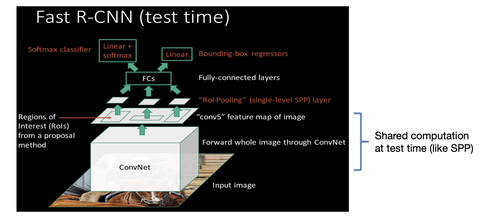
RoI Pooling RoI Pooling is a technique introduced in the Fast R-CNN framework to efficiently extract fixed-size feature representations for arbitrary regions(bounding boxes) in a feature map. It address the problem of feeding region proposals of various sizes into a neural network in a way that:
-
Preserves spatial information with each region of interest(RoI).
-
Produces a fixed-dimensional feature vector needed by fully connected layers(classifiers).
1. Feature extraction for the entire image
Instead of cropping individual region proposals from the original image and passing them each though a ConvNet(as done in older approaches like R-CNN), we:
-
Feed the entire image into a convolutional neural network(e.g., VGG, ResNet).
-
Obtain the resulting feature map, typically a 2D grid of activations.
This means the network only processes the image once, which is much more efficient.
2. Mapping region proposals to the feature map
You have a set of region proposals(bounding boxes) in the original image coordinates-these come from an external region proposal method(e.g., selective search) or from a region proposal network(in Faster R-CNN).
Each region proposal is then mapped onto the feature map coordinates:
- Because the CNN reduces spatial resolution(due to pooling layers or strided convolutions), the coordinates of each region of the original image need to be scaled to align with the coordinate system of the smaller feature map.
3. Dividing each RoI into Sub-regions
To handle different RoI sizes but produce a fixed-size output(for example 7X7 output grid in Fast R-CNN):
-
Divide the mapped RoI on the feature map into a predefined grid(e.g., 7X7).
-
Each sub-region in this grid corresponds to a smaller set of feature map cells.
4. Pooling operation
Within each of these sub-regions(bins):
-
Perform a pooling operation(usually max pooling, though average pooling can also be used).
-
This operation collapses the variable-sized sub-region into a single value(e.g., the maximum activation within that bin).
By doing this for each subregion in the grid, you transform the entire RoI into a fixed-size feature map(e.g., 7X7), regardless of the original size of the bounding box.
5. Feeding pooled features to classifier layers
Note that you have a fixed spatial dimension(e.g., 7X7), you can:
-
Flatten or otherwise reshape this pooled feature map.
-
Pass it into fully connected layers(and ultimately classification/regression heads) to predict:
- The object class for that region.
- The bounding box refinement offsets, etc.
Result of Fast R-CNN
Faster R-CNN
Faster R-CNN = Fast R-CNN + Region proposal network
Region Proposal Network: We fix the number of proposals by using a set of anchors per location.
A 256-d descriptor characterizes every location.
For feature map location, we get a set of anchor corrections and classification into object/non-object.
RPN: Training
Classification ground truth: We compute which indicates how much an anchor overlaps with the ground truth bounding boxes:
-
1 indicates that the anchor represents an object(foreground), and 0 indicates a background object. The rest do not contribute to the training.
-
For an image, randomly sample a few(e.g., 256) anchors to form a mini-batch(balanced objects vs. non-objects)
-
We learn anchor activate with the binary cross-entropy loss
-
Those anchors that contain an object are used to compute the regression loss.
-
Each anchor is described by the center position, width and height().
-
What the network actually predicts are:
\[\begin{equation} t_x = \frac{x - x_a}{w_a}
\end{equation}]
\[\begin{equation} t_y = \frac{y - y_a}{h_a}
\end{equation}]
\[\begin{equation} t_w = \log\!\biggl(\frac{w}{w_a}\biggr)
\end{equation}]
\[\begin{equation} t_h = \log\!\biggl(\frac{h}{h_a}\biggr)
\end{equation}]
-
Smooth L1 loss on regression targets
Faster R-CNN training:
- First implementation, training of RPN separate from the rest.
- Now we can train jointly!
- Four losses:
-
RPN classification(object/non-object)
-
RPN regression(anchor – proposal)
-
Fast R-CNN classification(type of object)
-
Fast R-CNN regression(proposal – box)
Feature Pyramid Networks
CNNs are not scale-invariant.
-
Idea A: Featurised image hierarchy
Featurised image hierarchy - Pros: Typically boosts accuracy(esp. at test time).
- Cons: Computationally inefficient.
-
Idea B: Pyramidal feature hierarchy
Pyramidal feature hierarchy - More efficient than Idea A, but
- Limited accuracy(inhibits the learning of deep representations)
-
Feature pyramid network(FPN)
Feature pyramid network - Higher scales benefit from deeper representation from lower scales.
- Efficient and high accuracy.
Straightforward implementation:
-
Convolution with 1 X 1 kernel
-
Upsampling(nearest neighbours)
-
Element-wise addition
Integration with RPN for object detection:
-
Define RPN on each level of the pyramid.
-
Only a single-scale anchor per level(scale varies across levels).
-
At test time, merge the predictions from all levels.
Pros:
-
Improves recall across all scales(esp. small objects).
-
More accurate(in terms of AP).
-
Broadly applicable, also for one-stage detectors.
-
Still in wide use today.
Cons: Increased model complexity.
Single-stage object detection
YOLO
-
Define a coarse grid().
-
Associate B anchors to each cell.
-
Each anchor is defined by:
- Localization(x, y, w, h).
- A confidence value(object/no object).
- And a class distribution over C classes.
Inference time:
It is more efficient than Faster R-CNN, but less accurate.
-
Coarse grid resolution, few anchors per cell = issues with small objects
-
Less robust to scale variation.
SSD
Pros:
-
More accurate than YOLO.
-
Works well even with lower resolution improved inference speed.
Cons:
-
Still lags behind two-stage detectors.
data augmentation is still crucial(esp. random sampling).
-
A bit more complex(due to multi-scale features).
RetinaNet
Problems with one-stage detectors
Two-stage detectors:
-
Classification only works on "interesting" foreground regions(proposals, 1-2k). Most background examples are already filtered out.
-
Class balance between foreground and background objects is manageable.
-
Classifier can concentrate on analyzing proposals with rich information.
Problems with one-stage detectors:
-
Many locations need to be analyzed(100k) densely covering the image - foreground-background imbalance.
- Many negative examples(every cell on the feature grid).
- Few positive examples(actual number of objects).
-
Hard negative mining: subsample the negatives with the largest error:
- works, but can be unstable.
Class imbalance:
- Idea: balance the positives/negatives in the loss function.
- Recall cross-entropy loss:
Focal loss
Replace CE with focal loss(FL):
-
When , it is equivalent to the cross-entropy loss.
-
As goes towards 1, the easy examples are down-weighted.
-
Example: , if , FL is lower than CE.
RetinaNet
-
One-stage(like YOLO and SSD) with Focal Loss.
-
Feature extraction with ResNet.
-
Multi-scale prediction - now with FPN.
Spatial Transformers
Features of Spatial pooling:
-
Helps detect the presence of features.
-
No information about precise location of features within a RoI.
- No effect on the RoI localization.
Solution: Spatial Transformers.
Equivariance is needed:
-
Learn to predict the parameters of the mapping :
Spatial Transformers -
Learn to predict a chain of transformations.
-
Learn to localize RoI without dense supervision(only class label).
-
Training multiple STs: Focus on different object parts.
-
Learning to localize without any supervision.
-
Makes the network equivariant to certain transformers(e.g., affine).
-
Fully differentiable.
Cons:
- Difficulty of training for generalizing to more challenging scenes.
Detection evaluation
Precision: How many zebras you found are actually zebras?
Recall: How many actual zebras in the image/dataset you could find?
What is a true positive?
-
Use the Intersection over Union(IoU).
-
e.g., if – positive match
-
The criterion is defined by the benchmarks(MS-COCO, Pascal VOC)
Resolving conflicts
-
Each prediction can match at most 1 ground truth box.
-
Each ground truth box can match at most 1 prediction.
All-in-one metric: Average precision(AP)
There is often a trade-off between Precision and Recall.
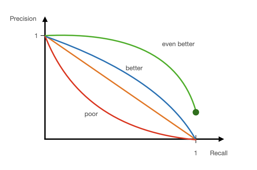
AP = the area under the Precision-Recall curve(AUC)
Computing average precision
-
Sort the predicted boxes by confidence score
-
For each prediction find the associated ground truth
- The ground truth should be unassigned and pass IoU threshold
-
Compute cumulative TP and FP:
- TP: [1, 0, 1] FP: [0, 1, 0] cTP = [1, 1, 2], cFP = [0, 1, 1]
-
Compute precision and recall(#GT = 3 TP + FN + 3)
- Precision: ; Recall(#GT=3):
-
Plot the precision-recall curve and the area beneath(num. integration).
mAP is the average over object categories
Single object tracking
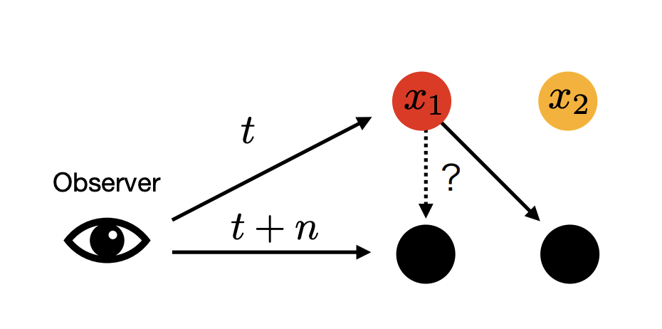
Problem statement: Given observations at , and find their correspondence at
Challenges:
-
Fast motion.
-
Changing appearance.
-
Changing object pose.
-
Dynamic background.
-
Occlusions.
-
Poor image quality.
-
...
A simple solution: Tracking by detection.
- Detect the object in every frame.
Problem: data association.
-
Many objects may be present & the detector may misfire.
-
We could use the motion prior.
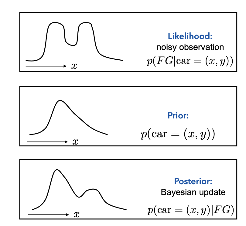
Bayesian tracking
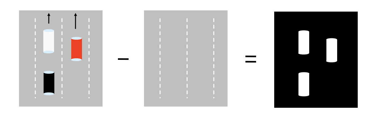
Goal: Estimate car position at each time instant (say, the white car).
Observation: Image sequence and known background.
-
Perform background subtraction.
-
Obtain binary map of possible cars.
-
But which one is the one we want to track?
Observations: Image
System state: Car position()
Notations:
-
: internal state at k-th frame
- Hidden random variable, e.g., position of the object in the image.
- history up to time step k.
-
: Measurements at k-th frame
- Observable random variable, e.g., the given image.
- history up tp time step k.
Goal:
Estimate posterior probability .
How? Recursion:
Hidden Markov model
Two assumptions of HMM:
Recursive Estimation
Key Concepts:
-
Bayes’ Rule:
-
Assumption:
-
Marginalization:
-
Factorization from graphical model:
Bayesian formulation:
Estimators:
Assume the posterior probability is known:
-
posterior mean:
-
maximum a posterior(MAP):
Deep networks:
-
It is easy to see what the networks have to output given the input
- but it is harder(yet more useful) to understand what a network models in terms of our Bayesian formulation.
-
Typically, the networks are tasked to produce MAP directly, e.g.,
without modeling the actual state distribution.
Online vs. Offline tracking
Online tracking:
- "Given observations so far, estimate the current state."
-
Process two frames at a time.
-
For real-time applications.
-
Prone to drifting hard to recover from errors or occlusions.
Offline tracking:
- "Given all observations, estimate any state."
-
Process a batch of frames.
-
Good to recover from occlusions(short ones as we will see)
-
Not suitable for real-time application.
-
Suitable for video analysis.
An online tracking model can be used for offline tracking too. Our recursive Bayesian model will still work.
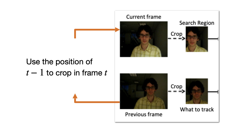
GOTURN
-
Input: Search region + template region(what to track).
-
Output: Bounding box coordinates in the search region.
Temporal prior:
where is Dirac delta function.
Advantages:
-
Simple: close to template matching.
-
efficient(real-time).
-
end-to-end(we can make use of large annotated data).
Disadvantages:
-
may be sensitive to the template choice.
-
the temporal prior is too simple: fails if there is fast motion or occlusion.
-
tracking one object only.
Online adaptation
Problem: The initial object appearance may change drastically,
- e.g., due to occlusion, pose change, etc.
Idea: adapt the appearance model on the (unlabeled) test sequence.
MDNet
Tracking with online adaptation

Multi-object tracking
Challenges:
-
Multiple objects of the same type.
-
Heavy occlusions.
-
Appearances of individual people are often very similar.
DL’s role in MOT:
-
Tracking initialization(e.g., using a detector.)
- Deep learning more accurate detectors.
-
Prediction of the next position(motion model).
- We can learn a motion model from data.
-
Matching predictions with detections:
- Learning robust metrics(robust to pose changes, partial occlusions, etc.).
- Matching can be embedded into the model.
Approach 1
-
Track initialization(e.g., using a detector).
-
Prediction of the next position(motion model).
- Classic: Kalman filter(e.g., state transition model.)
- DL(data driven): LSTM/GRU.
-
Matching predictions with detections(appearance model).
- In general: reduction to the assignment problem.
- Bipartite matching.
Typical models of dynamics
-
Constant position:
- i.e. no real dynamics, but if the velocity of the object is sufficiently small, this can work.
-
Constant velocity(possibly unknown):
- We assume that the velocity does not change over time.
- As long as the object does not quickly change velocity or direction, this is a quite reasonable model.
-
Constant acceleration(possibly unknown):
- Also captures the acceleration of the object.
- This may include both the velocity, but also the directional acceleration.
Bipartite matching
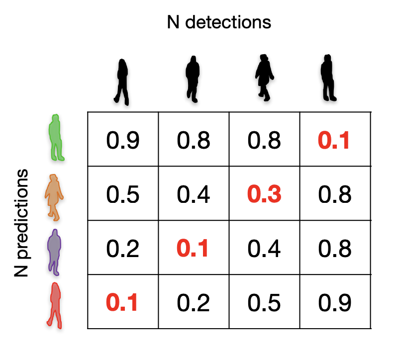
-
Define distances between boxes(e.g., 1 - IoU).
- We obtain matrix.
-
Solve the assignment.
- Using Hungarian algorithm
-
The bipartite matching solution corresponds to the minimum total cost.
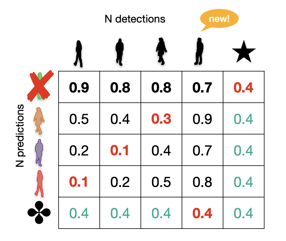
What happens if one detection is missing?
-
Add a pseudo detection with a fixed cost(e.g., 0).
-
Run the Hungarian method as before.
-
Discard the assignment to the pseudo node.
What happens if no prediction is suitable?
-
e.g., the object leaves the frame.
-
Solution: Pseudo node.
-
Its value will define a threshold.
-
We may need to balance it out.
Approach 2: Tracktor
-
Detect objects in frame (e.g., using an object detector)
-
Initialize in the same location in frame j.
-
Refine predictions with regression.
-
Run object detection again to find new tracks.
Advantages:
-
We can reuse well-engineered object detectors:
- The same architecture of regression and classification heads.
-
Work well even if trained on still images:
- The regression head is agnostic to the object ID and category.
Disadvantages:
-
No motion model:
- problems due to large motions(camera, objects) or low frame rate.
-
Confusion in crowded spaces:
- Since there is no notion of "identity" in the model.
-
Temporary occlusions(the track is "killed"):
- Generally applies to all online trackers.
- Partial remedy: Long-term memory of tracks(using object embeddings).
Problem of using IoU as metric:
The implicit assumption of small motion.
We need a more robust metric.
Metric learning: For re-identification(Re-ID)
Metric spaces
Definition:
A set (e.g., containing images) is said to be a metric space if with any two points and of there is associated a real number , called the distance from to , such that
Any function with these properties is called a distance function, or a metric.
Let’s reformulate:
-
We can decouple representation from the distance function:
- We can use simple metrics(e.g., L1, L2, etc) or parametric(Mahalanobis distance).
-
The problem reduces to learning a feature representation
How do we train a network to learn a feature representation
-
Choose a distance function, e.g., L2:
-
-
Minimize the distance between image pairs of the same person:
-
Metric learning method: add negative pairs.
- Minimize the distance between positive pairs; maximize it otherwise.
Our goal: .
The loss:
where and are sets of positive and negative image pairs.
-
Hinge loss:
- where is 1 if (A, B) is a positive pair, and 0 otherwise.
- hinge loss for negative pairs with margin
-
Triplet loss:
Triplet loss
Metric learning for tracking
-
Train an embedding network on triplets of data:
- positive pairs: same person at different timesteps;
- negative pairs: different people.
-
Use the network to compute the similarity score for matching.
Summary of metric learning
-
Many problems can be reduced to metric learning.
- Including MOT(both online and offline).
-
Annotation needed:
- e.g., same identity in different images.
-
In practice: careful tuning of the positive pair term vs. the negative term.
- hard-negative mining and a bounded function for the negative pairs help.
-
Extension to unsupervised setting - contrastive learning.
Online vs. Offline tracking
Online tracking:
- "Given observations so far, estimate the current state."
-
Process two frames at a time.
-
For real-time applications.
-
Prone to drifting hard to recover from errors or occlusions.
Offline tracking:
- "Given all observations, estimate any state."
-
Process a batch of frames.
-
Good to recover from occlusions(short ones as we will see)
-
Not suitable for real-time application.
-
Suitable for video analysis.
Graph based MOT
Tracking with network flow
Minimum-cost maximum-flow problem:
Determine the maximum flow with a minimum cost.
-
Node = object detection
-
Edge = temporal ID correspondence
-
Goal: disjoint set of trajectories
Minimizing the cost:
where is the disjoint set of trajectories, indicates the cost, and means the indicator .
To incorporate detection confidence, we split the node in two.
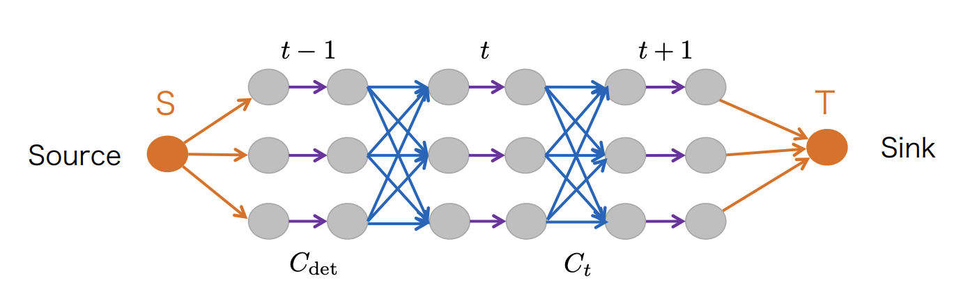
where indicates the detection confidence, and indicates the transition cost.
Problem with occlusions, such as:
-
occlusion in the last frame.
-
the object appears only in the second frame.
Solution: Connect all nodes(detections) to entrance/exit nodes:

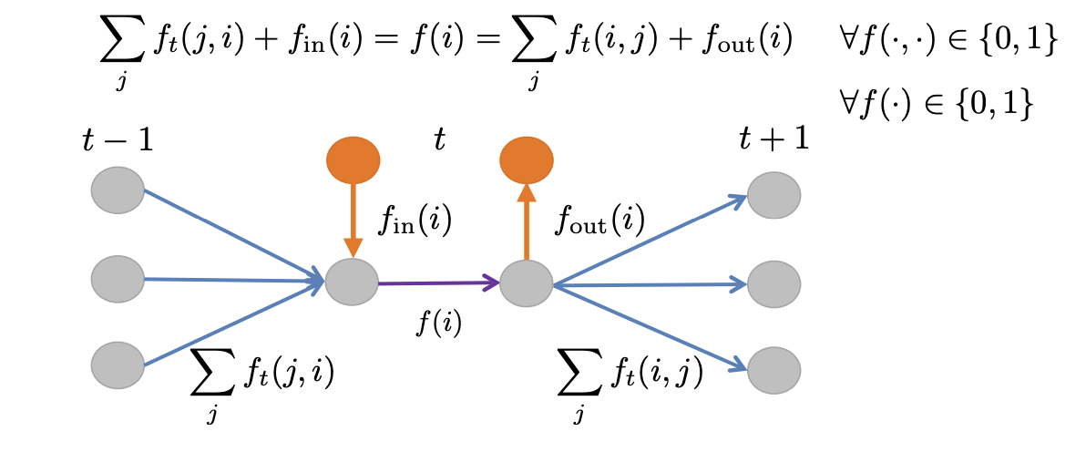
And the graph subjects to flow conservation:
MAP formulation
- Our solution is a set of trajectories
Bayes rule
Conditional independence of observations
Independence of trajectories
MAP fomulation:
Prior
Trajectory model: count the entrance, exit and transition costs
Entrance Cost:
Transition Cost:
Exit Cost:
Likelihood:
We can use Bernoulli distribution:
denotes prediction confidence (e.g., provided by the detector)
can be ignored in optimization
Optimization
() are estimated from data. Then:
-
Construct the graph from observation set .
-
Nodes (represent observations or potential assignments).
-
Edges (represent possible transitions between observations).
-
Costs assigned to edges.
-
Flow through the graph, which represents assignments.
-
-
Start with empty flow.
-
WHILE ( can be augmented):
-
Augment by one.
-
Find the min-cost flow by the algorithm of:
-
IF (current min cost global optimal cost):
- Store current min-cost assignment as global optimum.
-
-
Return the global optimal flow as the best association hypothesis.
Summary
-
Min-cost max-flow formulation:
the maximum number of trajectories with minimum costs.
-
Optimization maximizes MAP:
global solution and efficient(polynomial time).
Open questions:
-
How to handle occlusions
-
How to learn costs:
costs may be specific to the graph formulation and optimization.
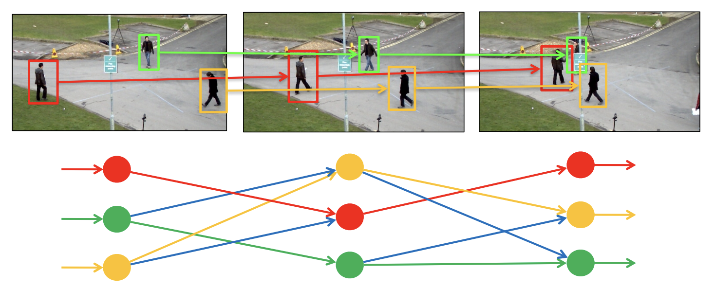
Tracking with Message Passing Network
End-to-end learning?
-
Can we learn features for multi-object tracking(encoding costs) to encode the solution directly on the graph?
-
Goal: Generalize the graph structure we have used and perform end-to-end learning.
Setup
-
Input: task-encoding graph
-
nodes: detections encoded as feature vectors
-
edges: node interaction(e.g., inter-frame)
-
-
Output: graph partitioning into(disjoint) trajectories
- e.g., encoded by edge label(0,1)
Deep learning on graphs
Key challenges:
-
Graph can be of arbitrary size
number of nodes and edges
-
Need invariance to node permutations.
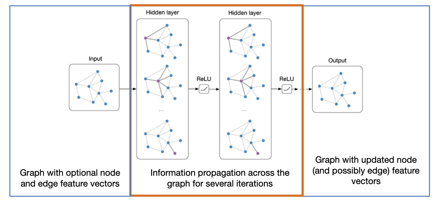
Message passing
-
Initial graph
-
Graph:
-
Initial embeddings:
- Node embedding:
- Edge embedding:
-
Embeddings after steps:
-
-
"Node-to-edge" update
Node-to-edge update -
"Edge-to-node" update
-
Use the updated edge embeddings to update nodes:
-
After a round of edge updates, each edge embedding contains information about its pair of incident nodes.
-
By analogy:
-
In general, we may have an arbitrary number neighbors("degree", or "valency")
-
Define a permutation-invariant aggregation function:
where the input is a set of embeddings from incident edges.
-
Re-define the edge-to-node updates for a general graph:
-
Remarks:
-
Main goal: gather content information into node and edge embeddings.
-
Is one iteration of node-to-edge/edge-to-node updates enough?
-
One iteration increases the receptive field of a node/edge by 1
- In practice, iterate message passing multiple times(hyperparameter).
-
All operations used are differentiable.
-
All vertices/edges are treated equally, i.i. the parameters are shared.
MOT with MPN

-
Input
-
Graph construction + feature encoding
- Encode appearance and scene geometry cues into node and edge embeddings.
-
Neural message passing
- Propagate cues across the entire graph with neural message passing.
-
Edge classification
- Learn to directly predict solutions of the Min-cost flow problem by classifying edge embeddings.
-
Output
Feature encoding
Appearance and geometry encodings:
-
Relative Box Position
-
This encodes the normalized relative position of two bounding boxes.
-
The difference in the y-coordinate is divided by the sum of their heights.
-
The difference in the x-coordinate is divided by the sum of their widths.
-
The factor 2 ensures the values are in a normalized range.
-
-
Relative Box Size
-
These terms encode the relative scale change between the two bounding boxes.
-
Using a logarithm makes it more robust to size differences.
-
-
Time Difference
-
This represents the time gap between the two detections.
-
It helps in determining whether two bounding boxes belong to the same object across frames.
-
*Shared weights of CNN and MLP for all nodes and edges
Contrast:
-
earlier: define pairwise and unary cost
-
now:
-
feature vectors associated to nodes and edges.
-
use message passing to aggregate context information into the features.
-
Temporal causality
Flow conservation at a node
-
At most 1 connection to the past.
-
At most 1 connection to the future.
Time-aware message passing:
Classifying edges
-
After several iterations of message passing, each edge embedding contains content information about detections.
-
We feed the embeddings to an MLP that predicts whether an edge is active/inactive
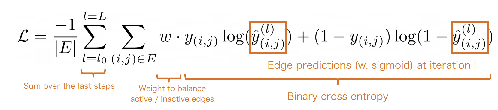
Obtaining final solutions
-
After classifying edges, we get a prediction between 0 and 1 for each edge in the graph.
-
Directly thresholding solutions do not guarantee flow conservation constraints.
-
In practice, around 98% of constraints are automatically satisfied.
-
Lightweight post-processing(rounding or linear programming).
-
The overall method is fast(12fps) and achieves SOTA in the MOT challenge by a significant margin.
Summary
-
No strong assumptions on the graph structure
- handling occlusions.
-
Costs can be learned from data.
-
Accurate and fast(for an offline tracker).
-
(Almost) End-to-end learning approach
- some post-processing is required.
Evaluation of MOT
Compute a set of measures per frame:
-
Perform matching between predictions and ground truth.
- Hungarian algorithm
-
FP = false positive
-
FN = false negative
-
IDSW = Identity switches
An identity switch (IDSW) happens in multi-object tracking (MOT) when the same object is assigned different IDs across frames. This means that the tracking system mistakenly reassigns a new ID to the same object, breaking continuity.
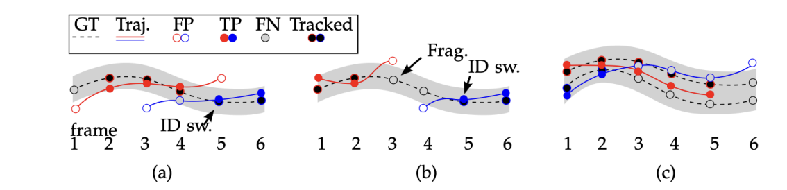
IDSW -
An ID switch is counted because the ground truth track is assigned first to red, then to blue.
-
Count both an ID switch(red and blue both assigned to the same ground truth), but also fragmentation(Frag.) because the ground truth coverage was cut.
-
Identity is preserved. If two trajectories overlap with a ground truth trajectory(within a threshold), the one that forces the least ID switches is chosen(the red one).
-
Metrics:
-
Multi-object tracking accuracy(MOTA):
-
score:
-
Multi-object tracking precision(MOTP):
Segmentation
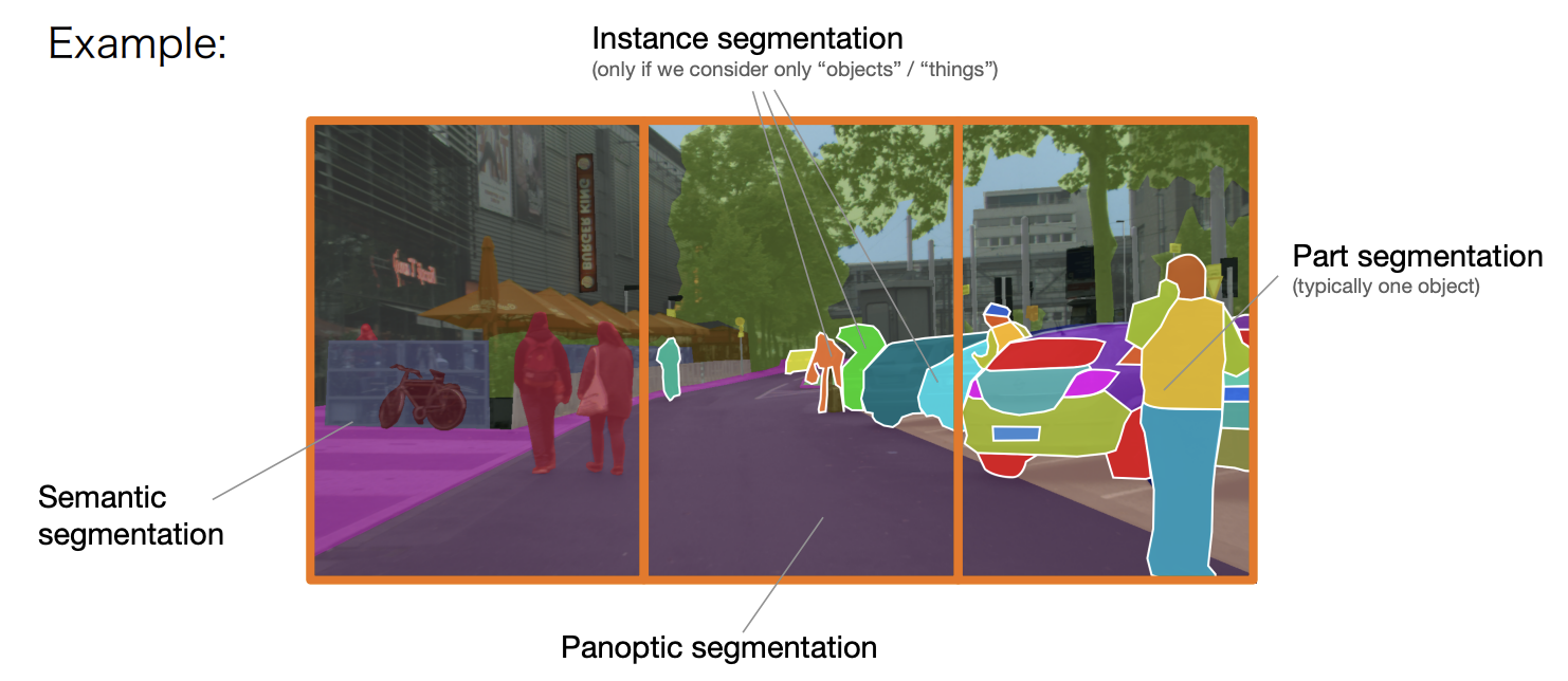
Flavors of image segmentation
-
Semantic segmentation: Label every pixel with a semantic category.
-
Instance segmentation: group object pixels as a separate category
-
Disregard background("stuff") classes, e.g., road, sky, building etc.
-
Can be class-agnostic or
-
with object classification: "semantic instance segmentation"
-
-
Panoptic segmentation: semantic + instance segmentation
-
Higher granularity, e.g., discriminating between object parts
- "part segmentation"
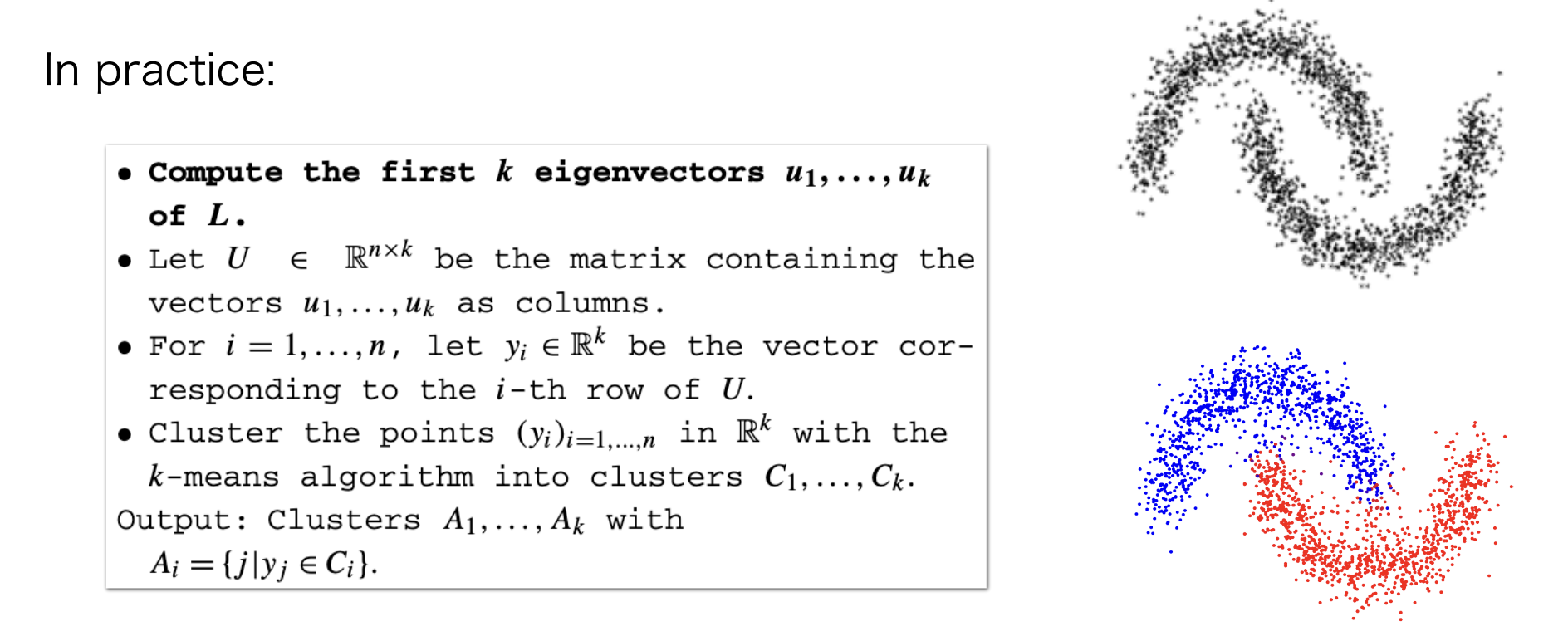
K-means(clustering)
-
Initialize(randomly) K cluster centers
-
Assign points to clusters
- using a distance metric
-
Update centers by averaging the points in the cluster
-
Repeat 2 and 3 until convergence.
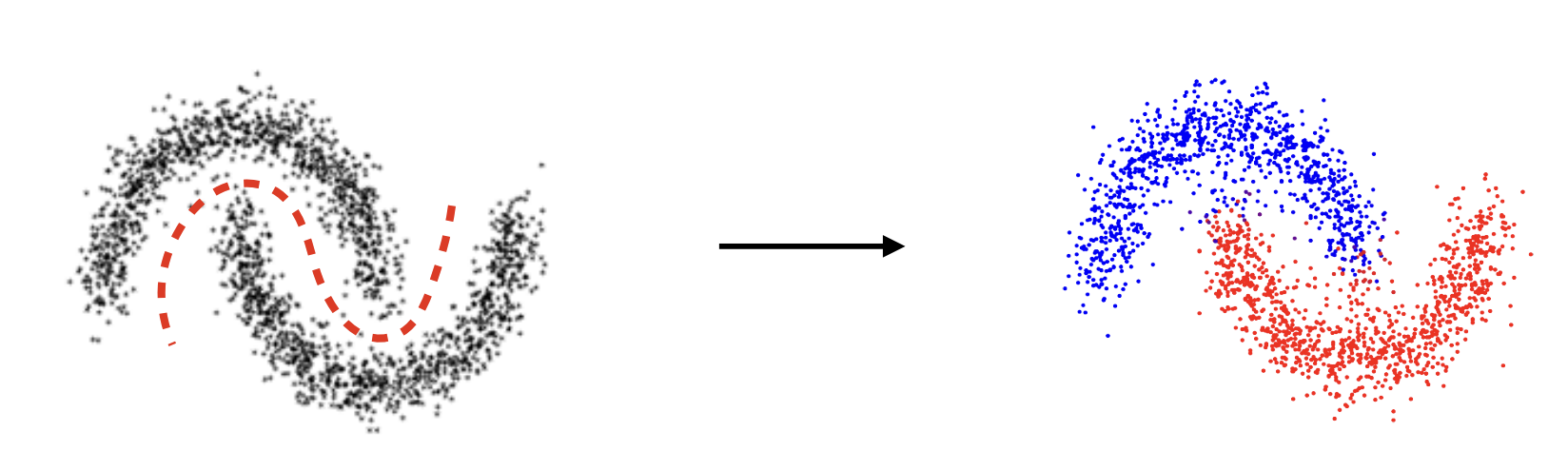
Problem: The Euclidean distance may be insufficient. Instead, we want to cluster based on the notion of "connectedness".
Spectral clustering
Construct a Similarity Graph:
-
Represent all data points as fully-connected(undirected) graph.
-
Edge weights encode proximity between nodes(Similarity Matrix).
-
measures the similarity of nodes and .
-
We can use a distance metric:
Compute the Graph Laplacian:
-
Define graph Laplacian:
where is a diagonal matrix(degree matrix):
Optimization problem:
The Laplacian quadratic form measures how much variation exists between connected nodes.
where
-
L is symmetric and positive semi-definite(L is positive semi-definite, meaning all its eigenvalues are non-negative().
-
If two points are highly connected, ( is large), then their values and should be similar, the term is small.
-
The goal is to minimize this sum, ensuring connected nodes have similar values.
-
The smallest eigenvectors of L correspond to smooth functions on the graph(meaning nodes in the same cluster should have similar values).
-
They reflect connected components or clusters in the graph.
Intuitively, if
then,
-
if (if and are in different clusters), then
-
if ( and are similar), then (same cluster)
The solutions are eigenvectors corresponding to the second smallest eigenvalues of .
Special case:
-
Zero eigenvalue
What can we say about the corresponding eigenvector?
-
Connected components
- Proposition: the multiplicity of eigenvalue 0 equals to the number of connected components, spanned by indicator vectors.
- Example with two components(:
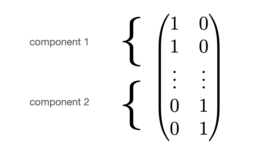
Example
-
Spectral clustering can handle complex distributions.
-
The complexity is due to eigendecomposition.
-
There are efficient variants(e.g., using sparse affinity matrices).
Normalized cut(Ncut)
Spectral clustering as a min cut as Fig 54
Problem with min cuts: Favour unbalanced isolated clusters:
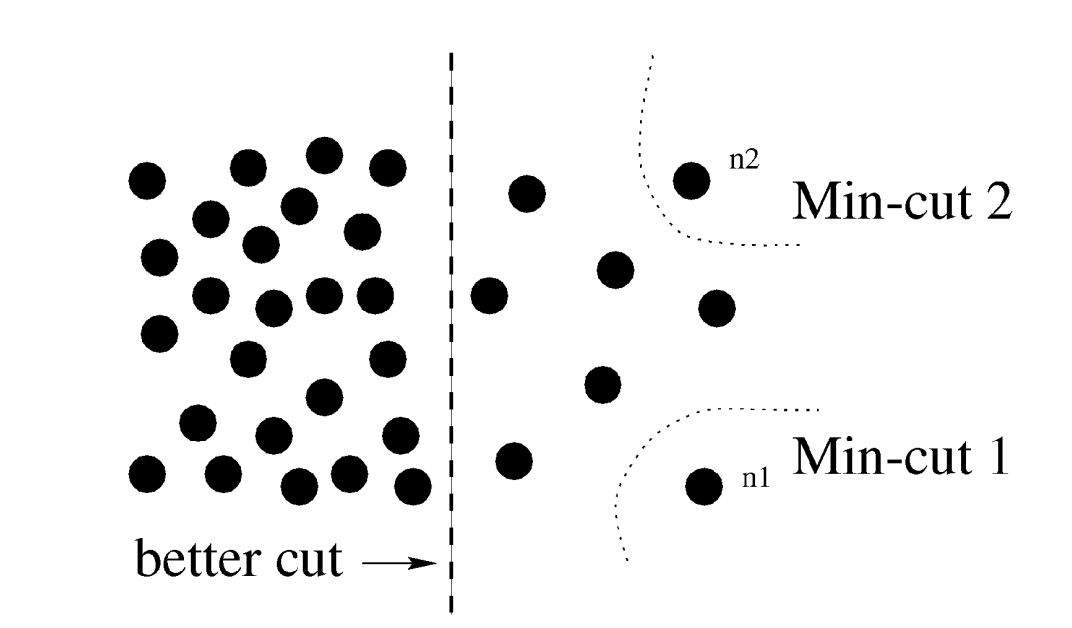
Balanced cut
where
-
The cost of cutting sets A and B:
-
Total edge cost in set A(equiv. B):
-
Intuitively - minimize the similarity between groups A and B, while maximizing the similarity within each group.
Ncut
-
Define a graph
-
V is the set of nodes representing pixels.
-
E defines similarities of two nodes.
-
-
Solves a generalized eigenvalue problem:
where
-
-
is the Laplacian matrix
-
equivalently
-
-
Use the eigenvector with the 2nd smallest eigenvalue to cut the graph.
-
Recurse if needed(i.e. subdivide the two node groups).
Energy-based model: Conditional random fields(CRFs)
Energy function:
where
-
is unary term
Unary potential:
-
encodes local information about a pixel.
-
how likely is it to belong to a certain class(e.g. foreground/background)
-
-
is the pairwise term.
Pairwise potential:
-
encode neighborhood information
-
how different is this pixel/patch to its neighbors(e.g. based on color/texture/learned feature)?
-
Conditional Random Fields
Boykov and Jolly (2001)
Variables
-
: Binary variable
- foreground/background
-
: Annotation
- foreground/background/empty
Unary term
-
-
Pay a penalty for disregarding the annotation
Pairwise term
-
-
Encourage smooth annotations
-
affinity between pixels and
Optimization with graph cuts:
Grid structured random fields
-
Efficient solution using Maxflow/Mincut
-
Optimal solution for binary labelling
Fully connected models:
-
Efficient solution using mean-field:
Variational methods.
Using fully connected CRFs:
Fully convolutional neural networks
Deep networks for classification:
To extend this to segmentation:
-
Remove GAP:
-
Increase number of parameters
-
Fixed input size only
-
No translation invariance
-
-
Replace fully connected layer with convolution( convolution)
-
Few parameters
-
Variable input size
-
Translation invariance
-
-
Upsample the last layer output to the original resolution.
-
Can be trained with pixel-wise cross-entropy with SGD.
convolution
-
Every (feature) pixel is a multi-dimensional feature.
-
convolution is equivalent to applying a shared fully connected layer to every pixel feature.
-
convolution is a pixel-wise linear projection:
-
each pixel is treated the same(shared parameters)
contrast this to a convolution
-
the output is treated as in fully connected layers:
followed by normalization, non-linearity(except for the output layer).
We may try to maintain the original image resolution in the encoder:
Output stride: input resolution/output resolution.
Decreasing the output stride improves segmentation accuracy.
The problems of keeping feature resolution high in all layers:
-
Receptive field size(replace stride-2 ops with dilation-2 ops):
-
Removing an operation with stride 2 reduces the area of the receptive field by a factor of 4̃.
-
Limited access to the context information.
-
-
Computational footprint(both memory and FLOPs):
- e.g., feature tensor size increases 4 times for each remove stride-2 operation.
Dilated convolutions: To maintain the receptive field size.
-
Consider convolution as a special case with "dilation" = 1:
-
For dilation N, the kernel "skips" pixels in-between:
Dilated convolution -
The number of parameters remains the same.
-
The receptive field size of kernel size and dilation "D":
-
Dilation improves scale invariance:
- we can use multiple dilations in the same layer.
ASPP
Problem 2: Computational footprint(both memory and FLOPs):
Solution: Upsampling
Recall convolution(as matrix multiplication):
We can obtain the opposite effect(increase the output size) by:
-
-
-
-
For CNNs, also apply the inverse of im2col to obtain the 2D grid representation - sums up overlapping values.
Transposed convolution:
-
Also called "up-convolution" or "deconvolution"(incorrect).
-
Pad each pixel in the input(e.g., zeros).
-
Convolve with a kernel(e.g., )
-
The amount of padding and stride determines the output resolution.
-
Equivalent implementation without padding:
Equivalent impl. -
Issue: Checkerboard Artifacts:
- Reason: Uneven overlap when kernel size is not divisible by stride.
Upsampling: Interpolation
-
Transposed convolution needs careful parameterization
- the boundaries can be still an issue.
-
A better alternative:
- Interpolation(e.g., bilinear) followed by standard convolution.
Resize-convolution:
-
Transposed convolution produces checkerboard artifacts
- can be resolved by a careful choice of the kernel/stride.
-
"Out-of-box" solution: interpolation, then convolve.
-
Issue: We still lost some information due to downsampling.
-
In general, there are multiple plausible results of upsampling.
U-Net
To mitigate information loss, we apply the first layers in the encoder via a skip connection.
U-Net’s key unique features:
-
Encoder-Decoder Structure: U-Net follows a symmetric encoder-decoder architecture. The encoder captures context through a series of convolutional layers, while the decoder uses this context to localize by progressively upsampling the feature maps.
-
Skip Connections: One of U-Net’s defining features is the use of skip connections. These connections directly link corresponding layers in the encoder and decoder, allowing the model to retain fine-grained spatial information during the upsampling process.
-
Asymmetric Depth: The depth of the network is asymmetric, with the encoder portion consisting of downsampling layers and the decoder portion consisting of upsampling layers. This structure enables the model to effectively capture both global context and precise local features.
-
Heavy Use of Convolutions: U-Net heavily relies on convolutions for feature extraction and localization. It often uses small convolutional kernels, typically of size 3x3, to capture intricate details and reduce computational overhead.
-
Efficient and Data Augmentation-Friendly: U-Net was designed with limited training data in mind. It can achieve high performance even with relatively small datasets. Additionally, U-Net networks are often augmented with random transformations (e.g., rotations, scaling, etc.) to further improve robustness and performance.
-
Pixel-wise Classification: The output of U-Net is a pixel-wise classification, where each pixel in the input image is assigned a class label, making it ideal for segmentation tasks.
-
Loss Function: U-Net commonly uses a pixel-wise softmax loss function for multi-class segmentation or binary cross-entropy for binary segmentation tasks. The architecture can be easily adapted for different types of loss functions, depending on the problem.
-
Symmetry and Output Size: Due to the symmetric structure of the architecture, the size of the output is the same as the input, which is an important feature for segmentation tasks where the output needs to align with the input image pixel-wise.
SegNet
SegNet is a deep learning architecture primarily used for image segmentation tasks. It is similar to U-Net in that it uses an encoder-decoder structure, but it has some unique features that distinguish it.
-
Encoder-Decoder Architecture: SegNet also follows an encoder-decoder design. The encoder consists of a series of convolutional layers that extract features from the input image, while the decoder upsamples the feature maps to create the segmented output.
-
Max Pooling Indices for Upsampling: A key difference between SegNet and other architectures, like U-Net, is that SegNet uses max pooling indices from the encoder during the upsampling in the decoder. This technique allows for more accurate localization and better reconstruction of fine details during the decoding process.
-
Efficient Memory Usage: By storing only the max pooling indices instead of the pooled feature maps, SegNet reduces memory consumption during the upsampling process, making it more efficient than many other models.
-
Pixel-wise Classification: Like U-Net, SegNet outputs pixel-wise classification, making it ideal for tasks such as semantic segmentation where each pixel needs to be classified into a category.
-
Loss Function: SegNet typically uses cross-entropy loss for training, which is commonly used for segmentation tasks.
-
Applications: SegNet has been successfully applied to a variety of tasks, such as road scene understanding, medical image analysis, and other segmentation applications requiring precise delineation of object boundaries.
Best practices for segmentation
-
Keep feature resolution high
- output stride 8 is typical.
-
Use dilated convolution to keep the receptive field size high.
- context information is important.
-
Use skip connections between the encode and decoder.
- improves upsampling quality.
-
Use image-adaptive post-processing such as CRFs.
- improves segmentation boundaries
Instance segmentation
-
Label every pixel, including the background(sky, grass, road).
-
Does not differentiate between the pixels from objects(instances) of the same class.
-
Do not label pixels from uncountable objects("stuffs"), e.g., "sky", "grass", "road".
-
Differentiates between the pixels coming from instances of the same class.
Proposal based method: Mask R-CNN
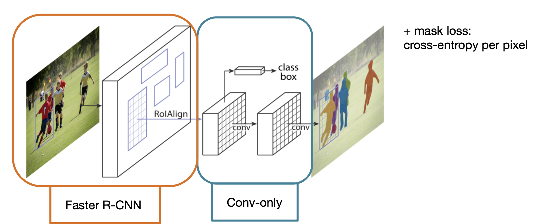
Start with Faster R-CNN
-
add another head "mask-head"
-
Mask R-CNN
-
Faster R-CNN + mask head for segmentation.
-
mask loss: cross-entropy per pixel.
-
New: RoIAlign
Mask R-CNN
RoIPool vs. RoIAlign
-
We need accurate localization for mask prediction.
-
RoIPool is inaccurate due to two quantization.
-
Better alternative: RoIAlign.
RoIAlign:
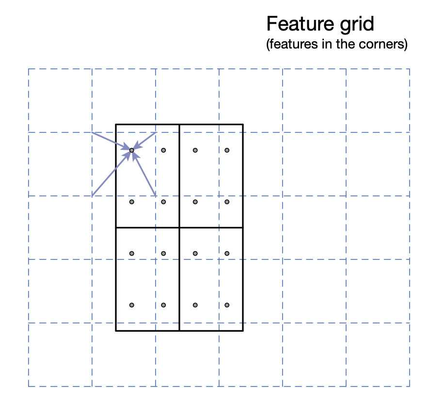
-
No quantization.
-
Define 4 regularly placed sample points within each bin.
-
Compute feature values with bilinear interpolation.
-
Aggregate each bin as before.
Problem of Mast R-CNN: Low mask resolution.
Mask R-CNN with PontRend
-
Mask head is an example of mapping a discrete signal representation(e.g., a pixel) to desired value(e.g., binary mask).
-
Instead, we parameterize the mask as a continuous function that maps the signal domain(e.g., (x, y) coordinate):
-
is an example of a coordinate-based net.
-
Why is it useful here?
-
We can query fractional coordinates
-
-
Idea:
-
Train coordinate-based mask representation by focusing on the boundaries.
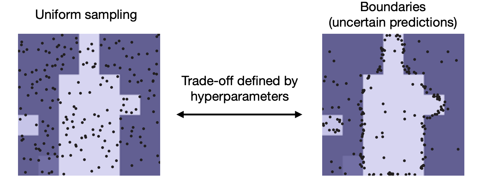
PointRend -
Test time: Use the learned coordinate mapping to refine boundaries.
-
-
Adaptive subdivision step(test time):
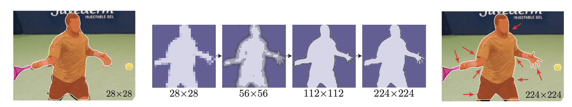
Qualitative result
Remarks:
-
In practice, compute a point-wise feature for each coordinate.
-
We compute a point-wise feature with bilinear interpolation.
-
We can concatenate features sampled this way from multiple feature maps.
-
The point head is trained on these features, not the coordinates.
-
Quiz: What’s the benefit?
Proposal-free method
We obtain a semantic map using Fully convolution networks for semantic segmentation.
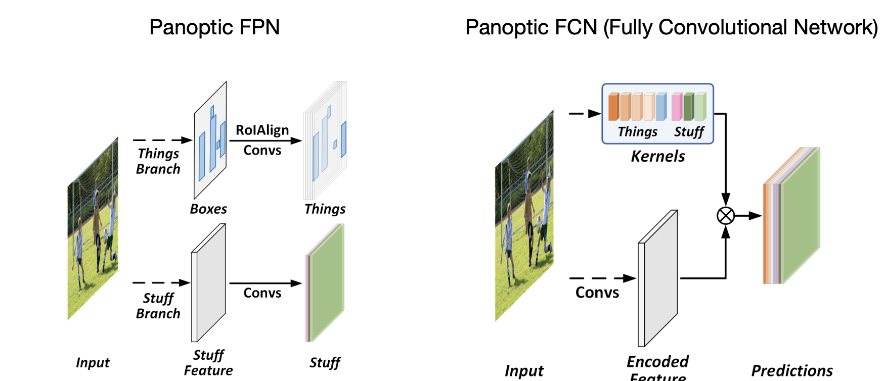
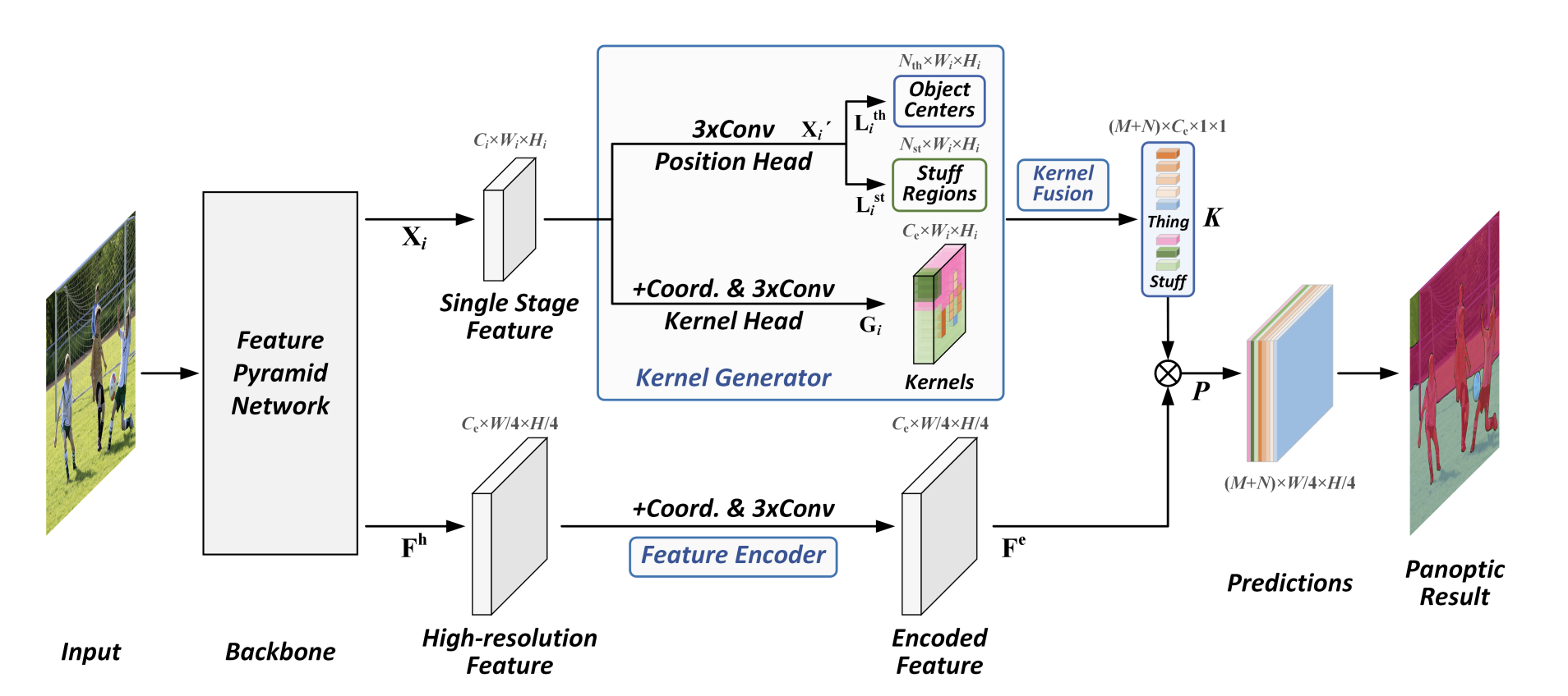
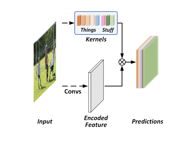
SOLOv2
-
Recall semantic segmentation.
-
The last layer is a convolution - a linear classifier:
-
: [] Pixel-wise class scores.
-
: [] Layer parameters( conv).
-
: [] Features.
-
-
Why not apply the same strategy to instance segmentation?
-
Problem: The number of kernels cannot be fixed.
Idea: Predict the kernels:
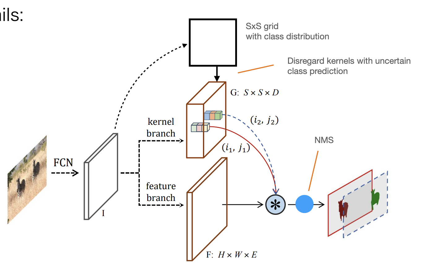
-
Convolution
-
Dimensionality depends on the kernel size( works well, so ).
Instance segmentation: Summary
-
Proposal-free and proposal-based instance segmentation methods offer accuracy vs. efficiency trade-off.
-
Similar to our conclusions about object detectors;
-
Proposal-based methods are more accurate(robust to scale variation), but less efficient;
-
Proposal-free methods are faster and have competitive accuracy.
Accurate segmentation of large-scale objects.
-
Panoptic segmentation
-
It gives labels to uncountable objects called "stuff"(sky, road, etc), similar to FCN-like networks.
-
It differentiates between pixels coming from different instances of the same class(countable objects) called "things"(cars, pedestrians, etc.).
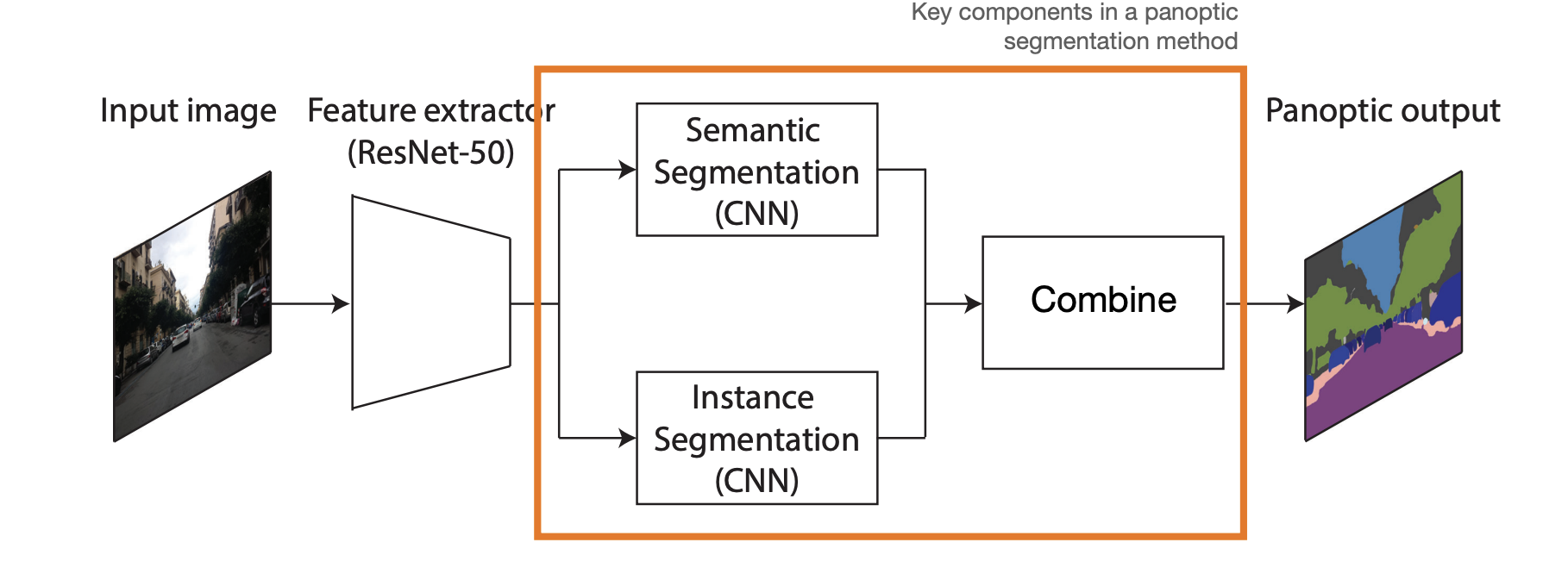
Challenges:
-
Can we harmonize architectures for predicting "Stuff" and "Things"?
- Semantic and instance segmentation pipelines are yet very different.
-
Can we improve computational efficiency via parameter sharing?
Two broad categories:
-
Top-down: typically two-stage proposal-based.
-
Bottom-up: learn suitable feature representation for grouping pixels.
Panoptic FPN
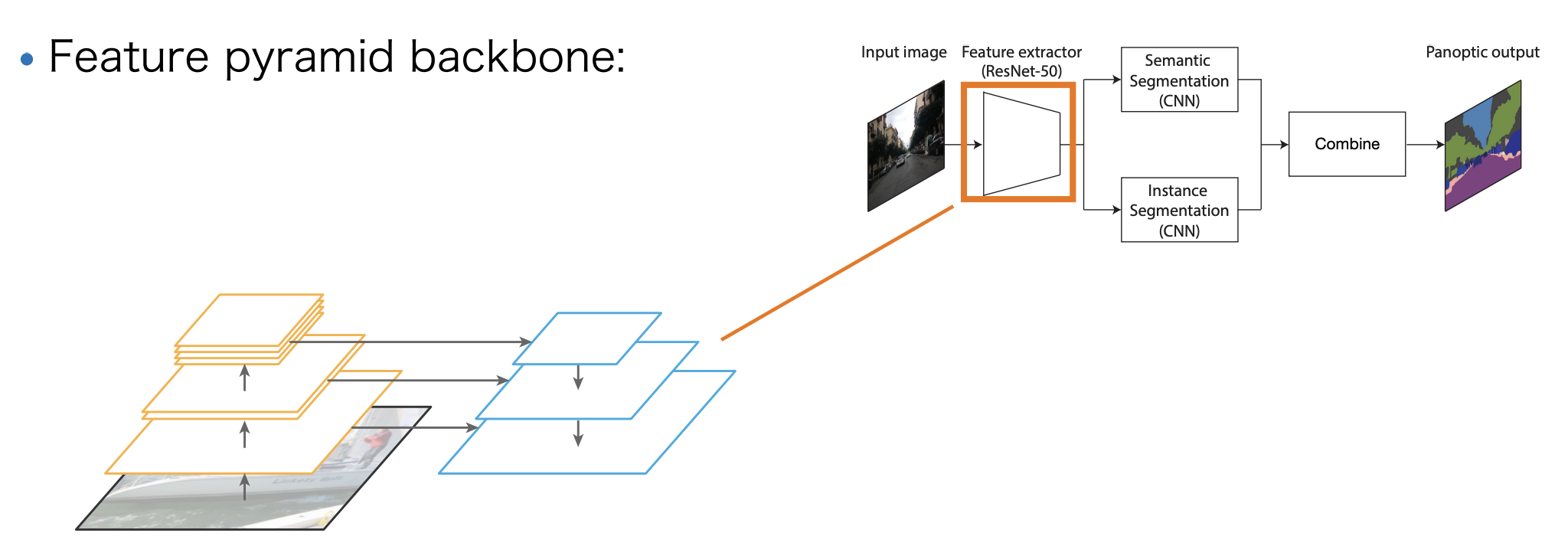
-
Feature pyramid backbone.
-
Mask R-CNN for instance segmentation.
-
Semantic segmentation decoder.
-
Replace things classes with 1 class "other".
-
Merge things and stuff:
-
NMS on instances.
-
Resolve stuff-things conflicts in favour of things.(WHY)
-
Remove any stuff regions labelled "other" or with a small area.
-
-
Loss function:
-
: Instance segmentation branch loss.
-
: Semantic segmentation branch loss.
-
: Trade-off hyperparameter.
-
Remark:
Training with multiple loss terms("multi-task learning") can be challenging, as different loss terms may "compete" for desired feature representation.
Panoptic FPN: Summary
-
Simple heuristic for merging things and stuff.
-
The instance and semantic segmentation branches are treated independently:
i.e., semantic segmentation branch receives no gradient from instance supervision and vice-versa.
Panoptic FCN
Even simpler?
Panoptic evaluation
Video object segmentation
Goal: Generate accurate and temporally consistent pixel masks for object in a video sequence.
Challenges:
-
Strong viewpoint/appearance changes.
-
Occlusions.
-
Scale change.
-
Illumination.
-
Shape.
-
…
What we need:
-
Appearance model:
-
Assumption: constant appearance.
-
Input: 1 frame.
-
Output: segmentation mask.
-
-
Motion model(maybe optional):
-
Assumption: smooth displacement; bright constancy.
-
Input: 2 frames.
-
Output: motion(optical flow).
-
Semi-supervised(one-shot) VOS task formulation:
-
Given: Segmentation mask of target object(s) in the first frame.
-
Goal: Pixel-accurate segmentation of the entire video.
-
Currently, the main testbed for dense(i.e. pixel-level) tracking.
-
Choosing the objects to track can be subjective(esp. online).
-
Offline tracking: considering the whole video - may provide a better clue(e.g., based on object permanence).
Motion-based VOS
Optical flow:
-
A pattern of apparent motion.
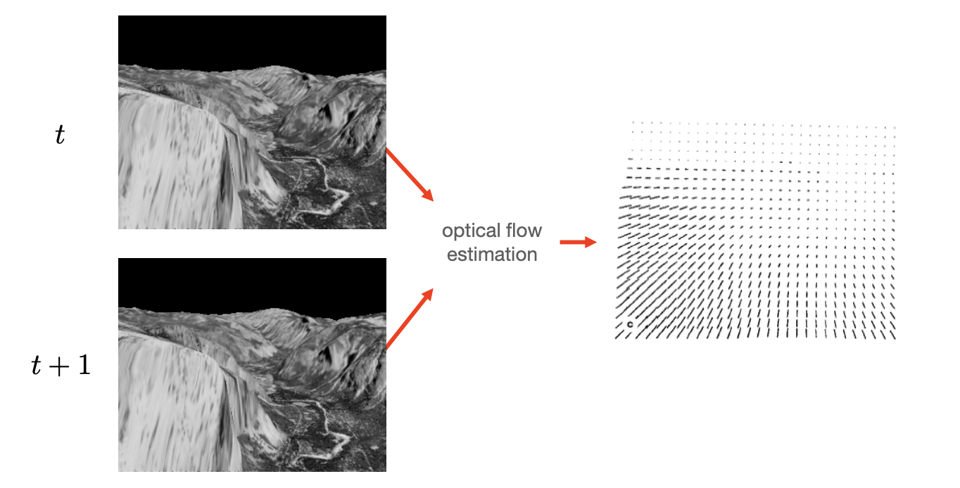
Optical flow -
Assumptions:
-
Brightness constancy:
Image measurements(brightness) in a small region remain the same.
-
Spatial coherence:
Neighbouring points in the scene typically belong to the same surface and hence typically have similar 3D motions.
-
Temporal persistence:
The image motion of a surface patch changes gradually over time.
-
Minimize brightness difference:
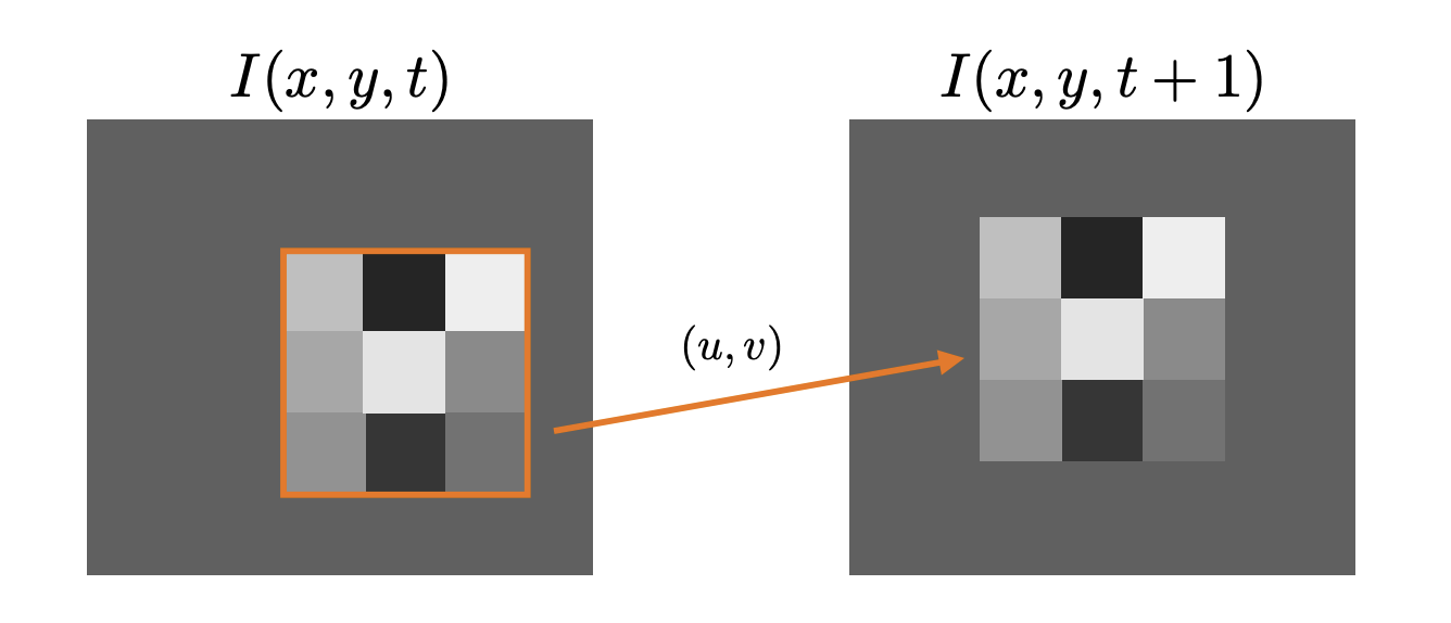
-
Goal: find minimizing:
-
First-order Taylor approximation of :
-
Differentiate w.r.t. and :
-
By rearranging the terms, we get a system of 2 equations with 2 unknowns:
-
By rearranging the terms, we get a system of 2 equations with 2 unknowns:
-
Structure tensor is positive definite, hence invertible, so
Lucas-Kanade:
This is a classical flow technique - Lucas-Kanade method.
Joint formulation of segmentation and optical flow estimation:
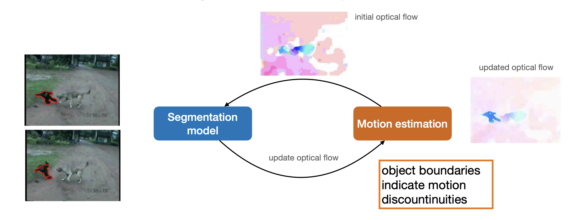
-
Joint formulation:
iteratively improving segmentation and motion estimation.
-
Slow to optimize:
runtime: up to 20s(excluding OF).
-
Initialization matters:
we need(somewhat) accurate initial optical flow.
-
DL to the rescue?
FlowNet: Architecture 1
-
Stack both(2) images input is now channels.
FlowNet -
Training with L2 loss from synthetic data.
FlowNet: Architecture 2 Siamese architecture
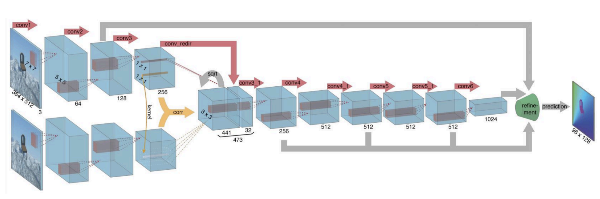
Correlation layer:
-
The dot product measures similarity of two features.
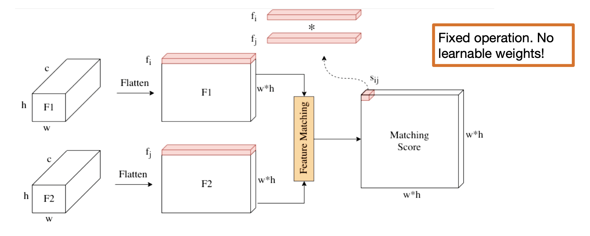
Correlation layer -
Correlation layer is useful for finding image correspondences.
-
SegFlow: Joint estimation of optical flow and object segment.
-
Joint feature representation at multiple scales.
-
Supervision need not be synchronized.
-
Motion-based VOS: Summary
-
We can obtain accurate estimates of optical flow with low latency.
-
Naively applying optical flow to dense tracking has limited benefits:
-
Due to severe (self-)occlusions, illumination changes, etc.
-
Still an active area of research in semi-supervised VOS(dense tracking).
-
-
Motion-based segmentation in a completely unsupervised setting:
Appearance-only VOS
Main idea:
-
Train a segmentation model from available annotation(including the first frame).
-
Apply the model to each frame independently.
One-shot VOS(OSVOS): Separate the training steps
-
Pre-training for "objections".
-
First-frame adaptation to specific object-of-interest using fine-tuning.
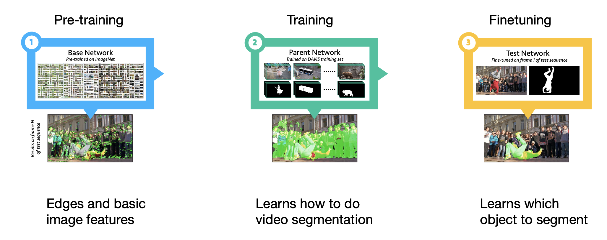
-
One-shot: learning to segment sequence from one example(the first frame).
-
This happens in the fine-tuning step:
the model learns the appearance of the foreground object.
-
After fine-tuning, each frame is processed independently no temporal information.
-
The fine-tuned parameters are discarded before fine-tuning for the next video.
Drifting problem:
-
The object appearance changes due to the changes in the object and camera pose
-
One idea: adapt the model to the video using pseudo-labels.
OnAVOS: Online Adaptation
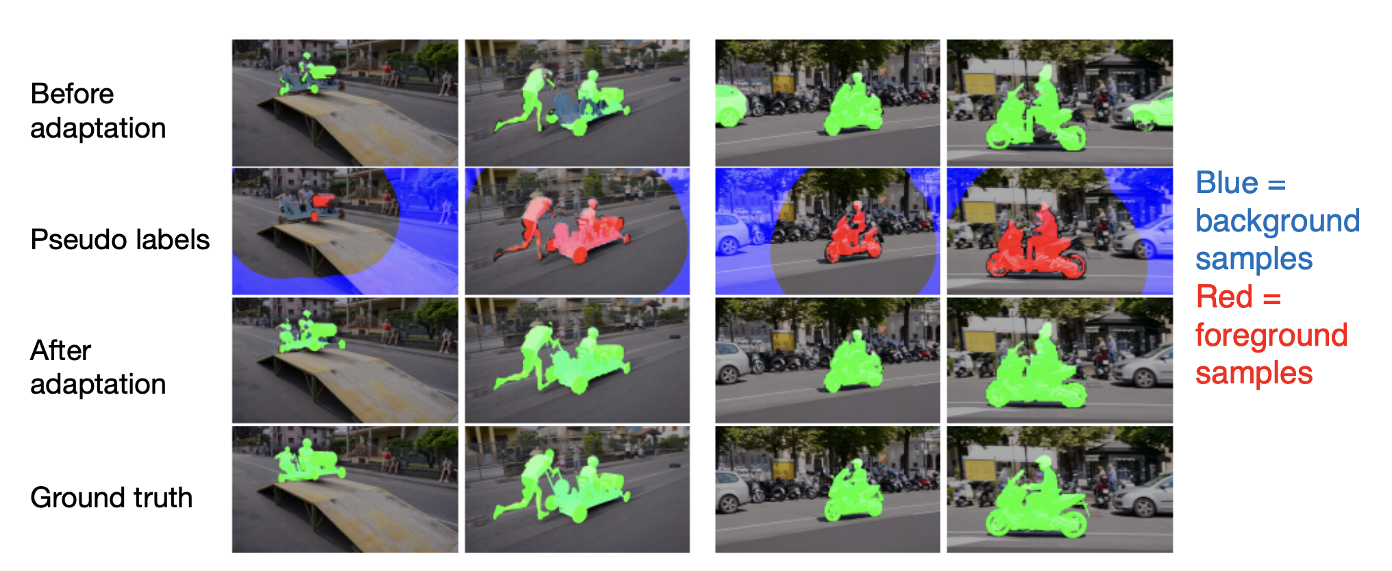
-
Adapt model to appearance changes in every frame, not just the first frame.
-
Drawback: can be slow.
-
OnAVOS is more accurate than OSVOS.
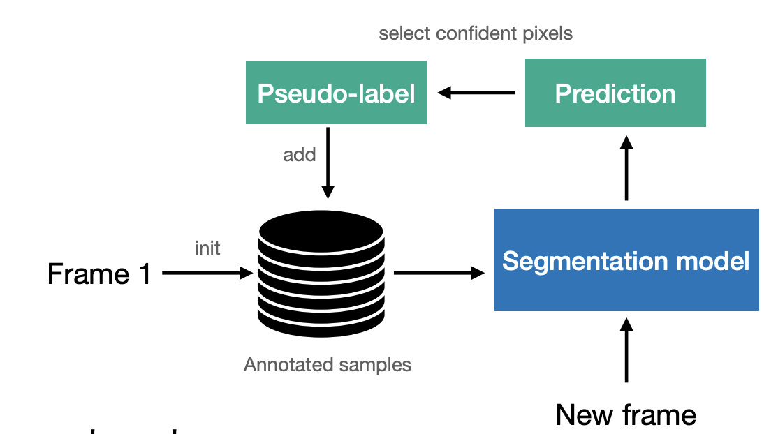
Online adaptation -
Instead of fine-tuning on a single sample, we fine-tune on a dynamic set of pseudo-labels.
-
The pseudo-labels may be inaccurate, so their benefit is diminished over time.
-
Next: A reverse approach: fine-tune the model with a correct signal.
MaskTrack
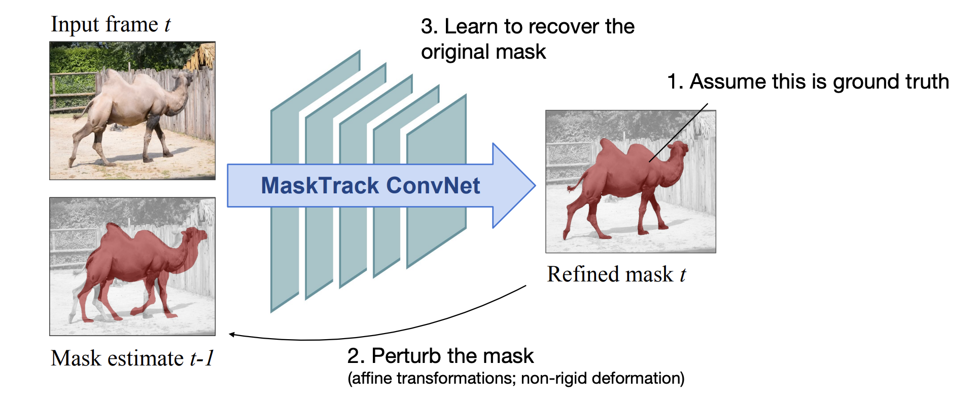
Traning inputs can be simulated
-
Like displacements to train the regressor of Faster R-CNN.
-
Very similar in spirit to Tracktor(Lecture 4)
Appearance-only VOS: Summary
Advantages of appearance-based models:
-
Can be trained on static images.
-
Can recover well from occlusions.
-
Conceptually simple.
Disadvantages:
-
No temporal consistency.
-
Can be slow at test-time(need to adapt).
Metric-based approaches
Pixel-wise retrieval:
-
Idea: Learn a pixel-level embedding space where proximity between two feature vectors is semantically meaningful.
-
The user input can be in any form, first-frame ground-truth mask, scribble....
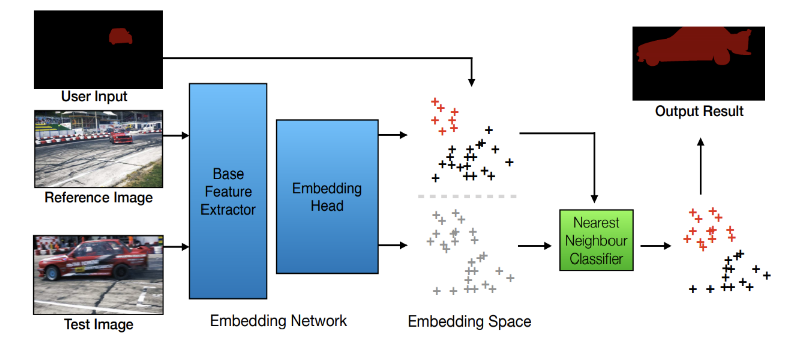
Pixel-wise retrieval -
Training: Use the triplet loss to bring foreground pixels together and separate them from background pixels.
-
Test: embed pixels from both annotated and test frame, and perform a nearest neighbor search for the test pixels.
-
Advantages:
-
We do not need to retrain the model for each sequence, nor fine-tune.
-
We can use unsupervised training to learn a useful feature representation(e.g., contrastive learning).
-
Transformers
CNNs: A few relevant facts
-
CNNs encode local context information.
-
Receptive field increases monotonically with network depth
-
This enables long-range context aggregation.
-
Yet increased depth makes training more challenging.
-
-
We may benefit from more explicit(u.e. in the same layer) non-local feature interactions.
Universality: Developing components that work across all possible settings:
-
Consider other modalities(language, speech, etc.)
-
Modern deep learning is only partially universal, even in the contexts we have seen so far(detection and segmentation).
-
Transformers can be applied to language and images with excellent results in both domains.
Self-attention: A hash table analogy
Consider a hash table:
-
The query is n-dimensional.
-
Each key is n-dimensional vector.
-
Each value is m-dimensional vector.
-
A hash table is not a differentiable function(of values w.r.t. keys); it’s not even continuous.
- We can access any value if we know the corresponding key exactly.
-
How can we make it differentiable
- Differentiable soft look-up.
-
We can obtain an(approximate) value corresponding to the query:
-
encodes normalized similarity of the query with each key:
-
We can use standard operators in our DL arsenal: dot product and softmax
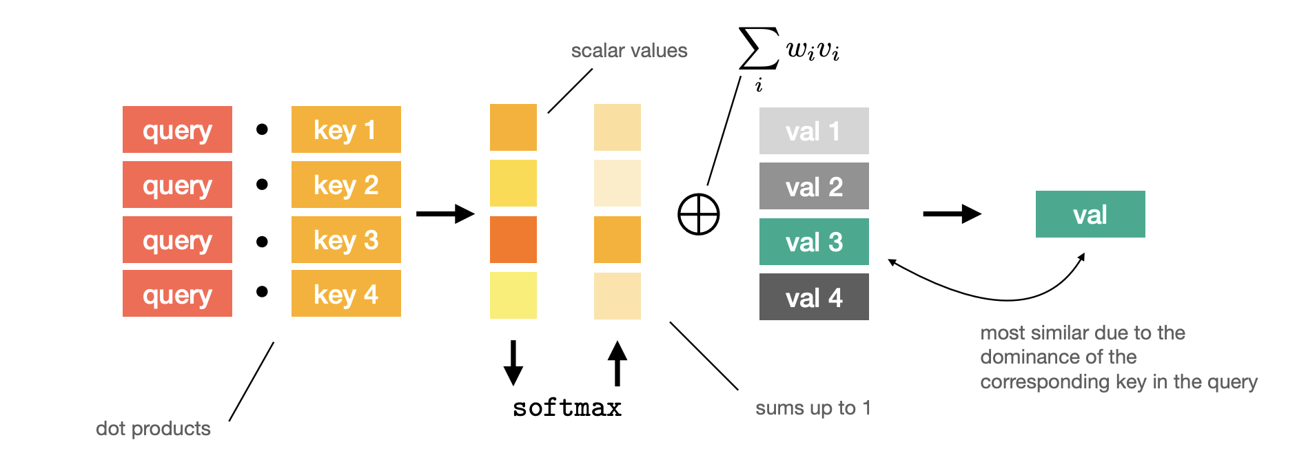
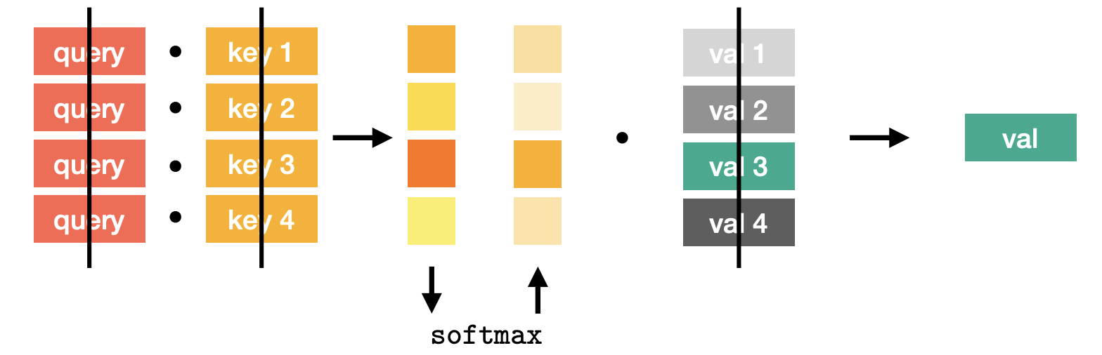
Self attention
Putting it all together:
-
A query vector : we have queries.
-
A key matrix : our hash table has (key, value) pairs.
-
A value matrix
Scaling factor eases optimization especially for large
-
Large increases the magnitude of the sum(we have n terms).
-
Values with large magnitude inside softmax lead to vanishing gradient.
Linear projection
-
Input: tokens of size
-
Define 4 linear mappings: , ,
-
Compute :
-
Output:
-
We started with [] and produced [] output
-
and all come form . This is called self-attention.
Complexity
-
Memory complexity():
-
Runtime complexity:
Multi-head attention
-
One softmax - one look-up operation.
-
We can extend the same operation to multiple look-ups without increasing the complexity.
-
This is called multi-heda attention.
-
Main idea: Chunk vectors
Multi-head - For example, split it in two(e.g., split 128d vectors into two 64d vectors).
-
Now we have two triplets, where feature dimension is reduced by a factor of 2.
-
Repeat the same process:
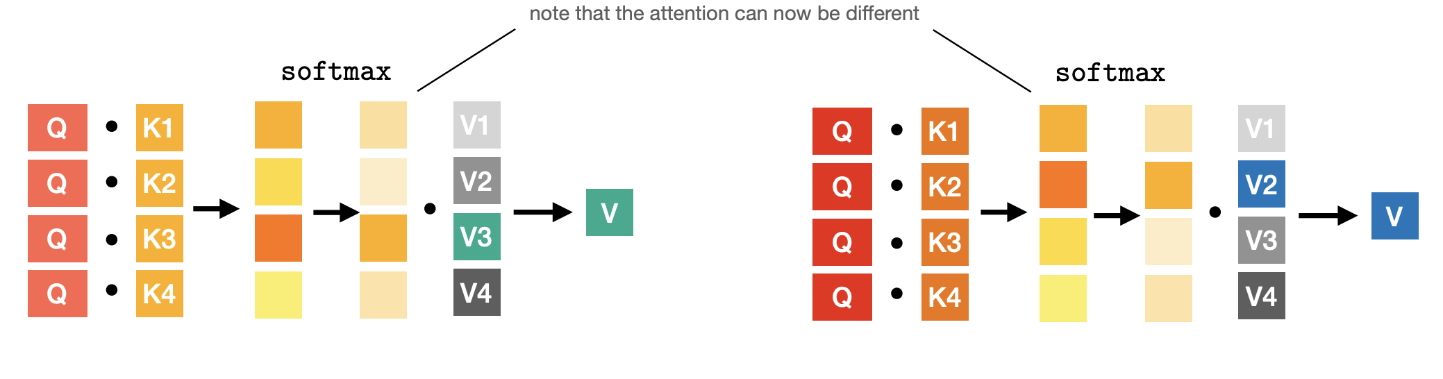
Multi-head -
Concatenate to obtain the original resolution.
-
Intuition: Given a single query, we can fetch multiple values corresponding to different keys.
-
We can design self-attention with arbitrary number of heads.
- condition: feature dimensionality of and should be divisible by it.
-
With heads, a single query can fetch up to different values.
- we can model more complex interactions between the tokens.
-
No increase in runtime complexity - actually faster in wall time.
Normalization:
Further improvements:
-
Residual connection:
add the original token feature before the normalization.
-
Layer normalization:
Normalize each token feature w.r.t. its own mean and standard deviation.
Recap:
-
Self-attention is versatile:
-
arbitrary number of tokens.
-
design choices: the number of heads, feature dimensionality.
-
-
Self-attention computation scales quadratically w.r.t. tokens
since we need to compute the pairwise similarity matrix.
-
Self-attention is permutation-invariant(w.r.t. the tokens):
-
the query index does not matter; we will always fetch the same value for it.
-
Is it always useful?
-
Transformers
Transformer-based encoder:
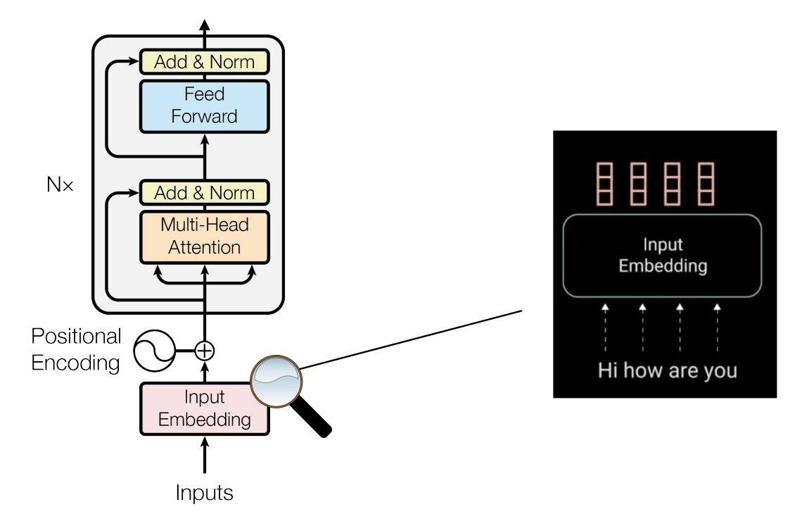
-
Positional encoding breaks permutation invariance.
-
Positional encoding is a matrix of size distinct values corresponding to each row.
-
Positional encoding stores a unique value(vector) corresponding to a token index.
-
It can be a learnable model parameter or fixed, for example:
-
It introduces the notion of spatial affinity(e.g., distance between two words in sentence; two patches in an image, etc.)
-
It breaks permutation invariance.
-
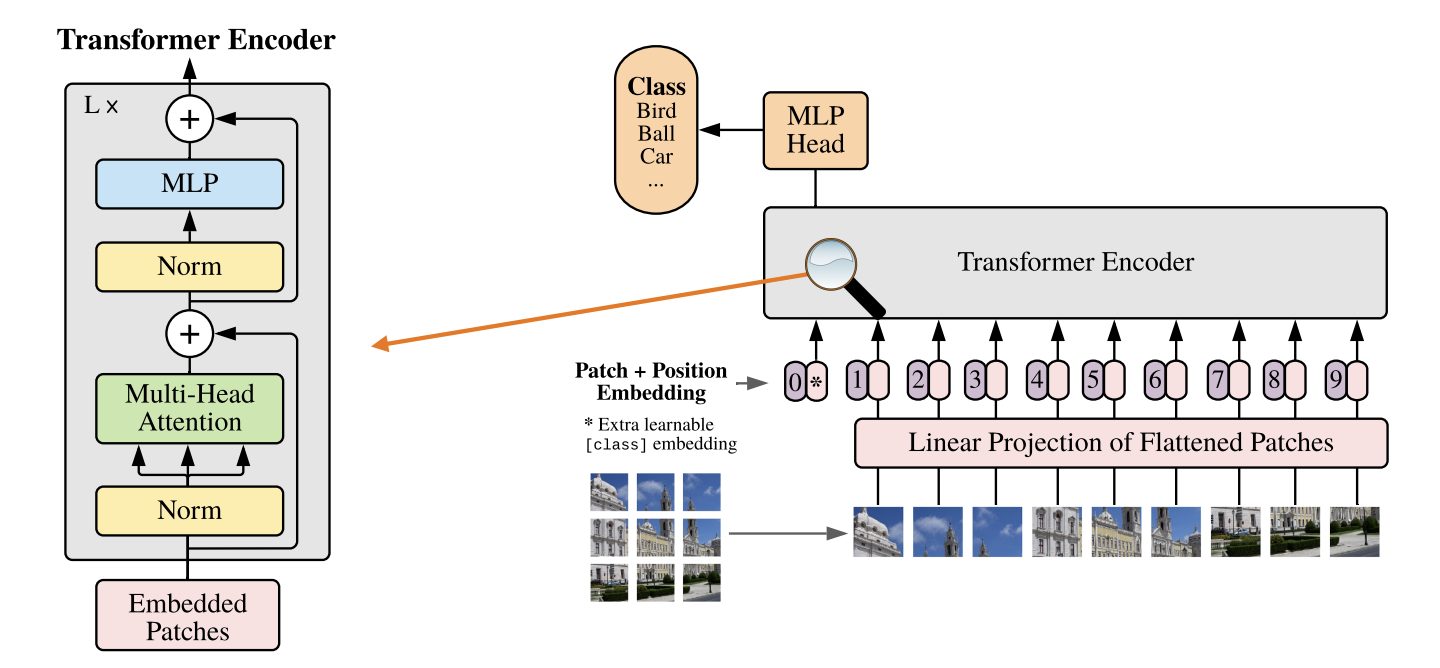
Vision Transformers
An all-round transformer architecture:
-
Competitive with CNNs(classification accuracy)*
-
Main idea: Train on sequences of image patches; only minor changes to the original(NLP) Transformer model.
-
Can be complemented with a CNN model
Steps:
-
Split an image into fixed-sized patches.
-
Linearly embed each patch(a fully connected layer).
-
Attach an extra "[class]" embedding(learnable).
-
Add positional embeddings.
-
Feed the sequence to the standard Transformer encoder.
-
Predict the class with an MLP using the output [class] token.
 ]
]
Experiment with ViT
-
ViT performs well only when pre-trained on large JFT dataset(300M images).(QUIZ: Why?)
-
ViT does not have the inductive biases of CNNs:
-
Locality(Self-attention is global.)
-
2D neighborhood structure(positional embedding is inferred from data.)
-
Translation invariance.
-
-
Nevertheless, now we use the same computational framework for two distinct modalities: Language and vision!
Swin Transformers
Recall ViT
-
We process patch embeddings with a series of self-attention layers:
- Quadratic computational complexity.
-
The number of tokens remains the same in all layers(QUIZ: How many/ what does it depend on?)
-
In CNNs, we gradually decrease the resolution, which has computation benefits(and increases the receptive field size).
-
Do ViT benefits from the same strategy?
Swin Transformer:
-
Construct a hierarchy of image patches.
-
Attention windows have a fixed size.
-
Linear computational complexity.
-
Output representation is compatible with standard backbones(e.g., ResNet).
- We can test many downstream tasks(e.g., object detection).
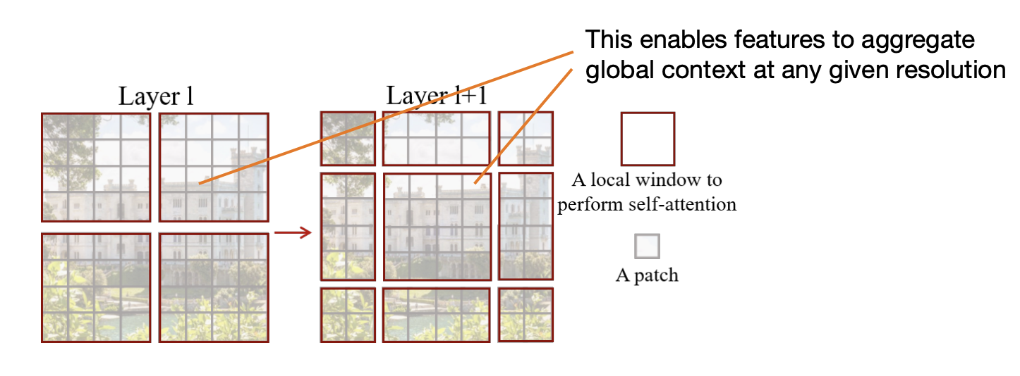
A naive implementation will hurt context reasoning:
At any given level(except the last one), our context is not global anymore:
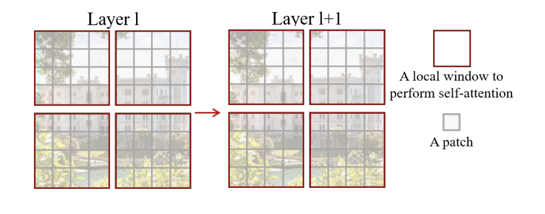
Solution: Alternate the layout of local windows:
Successively decrease the number of tokens using patch merging:
-
Concaternate C-dim patches into a feature vector (-dim);
-
Linearly transform to a dimensional vector.
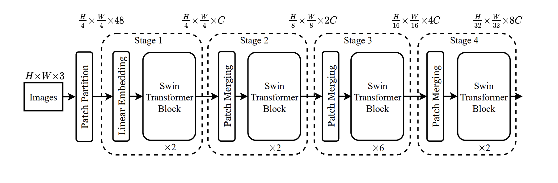
Results:
-
More efficient and accurate than ViT and some of CNNs(despite using lower resolution input).
-
Note: No pre-training on large datasets.
-
Improved scalability on large datasets(compare ImageNet-1K and ImageNet-22K)
Summary:
-
Reconciles the inductive biases from CNNs with Transformers;
-
State-of-the-art on image classification, object detection and semantic segmentation.
-
Linear computational complexity.
-
Demonstrates that Transformers are strong vision models across a range of classic downstream applications.
Transformer for detection?
-
Would it make sense to adapt the Transformer to object detection?
-
Recall that object detection is a set prediction problem:
- i.e., we do not care about the ordering of the bounding boxes.
-
Transformers are well-suited for processing sets.
-
Directly formulate the task as a set prediction!
DETR
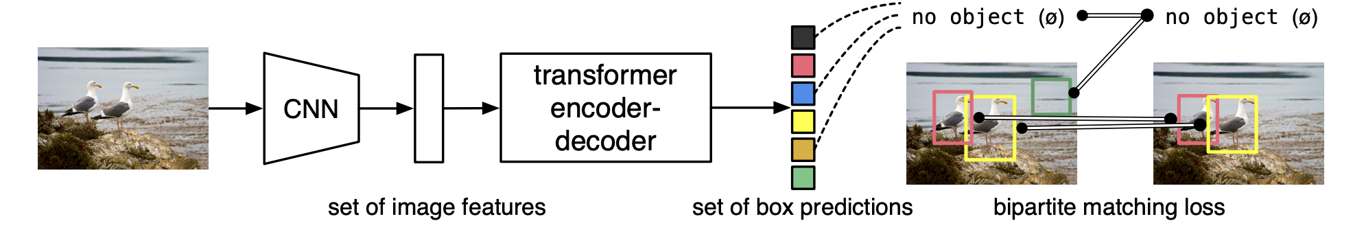
-
The CNN predicts local feature embeddings.
-
The transformer predicts the bounding boxes in parallel.
-
During training, we uniquely assign predictions to ground truth boxes with Hungarian matching.
-
No need for non-maximum suppression.
A closer look:
-
DETR uses a conventional CNN backbone to learn a 2D representation of an input image.
-
The model flattens it and supplements it with a positional encoding before passing it to the Transformer.
-
The Transformer encodes the input sequence.
-
TF encoder: "self-attention"
-
TF decoder: "cross-attention"
-
-
We supply object queries(laernable positional encoding) to the decoder, which jointly attends to the encoder output.
-
Each output embedding of the decoder is passed to a shared feed-forward network(FFN) that predicts either a detection(class and bounding box) or a "no object" class.

The losss function
where
-
: The total Hungarian loss used in DETR, which consists of classification and localization terms.
-
: The number of ground truth objects in the image.
-
: The predicted set of objects from the model.
-
: The ground truth set of objects.
-
: The optimal assignment of ground truth objects to predicted objects obtained using the Hungarian algorithm.
-
: The predicted probability for the class of the ground truth object assigned to prediction .
-
: The classification loss term, which penalizes incorrect class predictions.
-
: An indicator function that is 1 if the object is not the "no object" () class.
-
: The bounding box regression loss between the ground truth bounding box and the predicted bounding box .
The bounding box loss:
-
: A weight coefficient for the IoU (Intersection over Union) loss.(hyperparameter)
-
: The generalized IoU loss function, which penalizes misalignment between the predicted and ground truth bounding boxes.
-
: The ground truth bounding box for object .
-
: The predicted bounding box assigned to the ground truth object using the Hungarian algorithm.
-
: A weight coefficient for the L1 loss term.(hyperparameter)
-
: The L1 loss, which measures the absolute difference between the ground truth and predicted bounding box coordinates.
DETR: Summary
-
Accurate detection with a (relatively) simple architecture.
-
No need for non-maximum suppression.
- We can simply disregard bounding boxes with "empty" class, or low confidence.
-
Accurate panoptic segmentation with a minor extension.
-
Issues:
-
High computational and memory requirements(especially the memory).
-
Slow convergence / long training.
-
MaskFormer
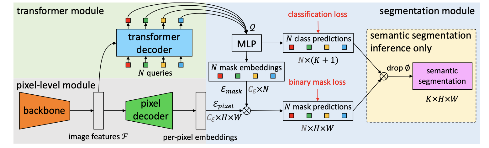
A unified model for semantic and panoptic segmentation.
Recall: Panoptic FCN
MaskFormer’s idea: Compute the kernels using learnable queries with a Transformer.
Works well, but has troubles with small objects/segments.
Mask2Former
Idea: Attend with self-attention at multiple scales of the feature hierarchy:
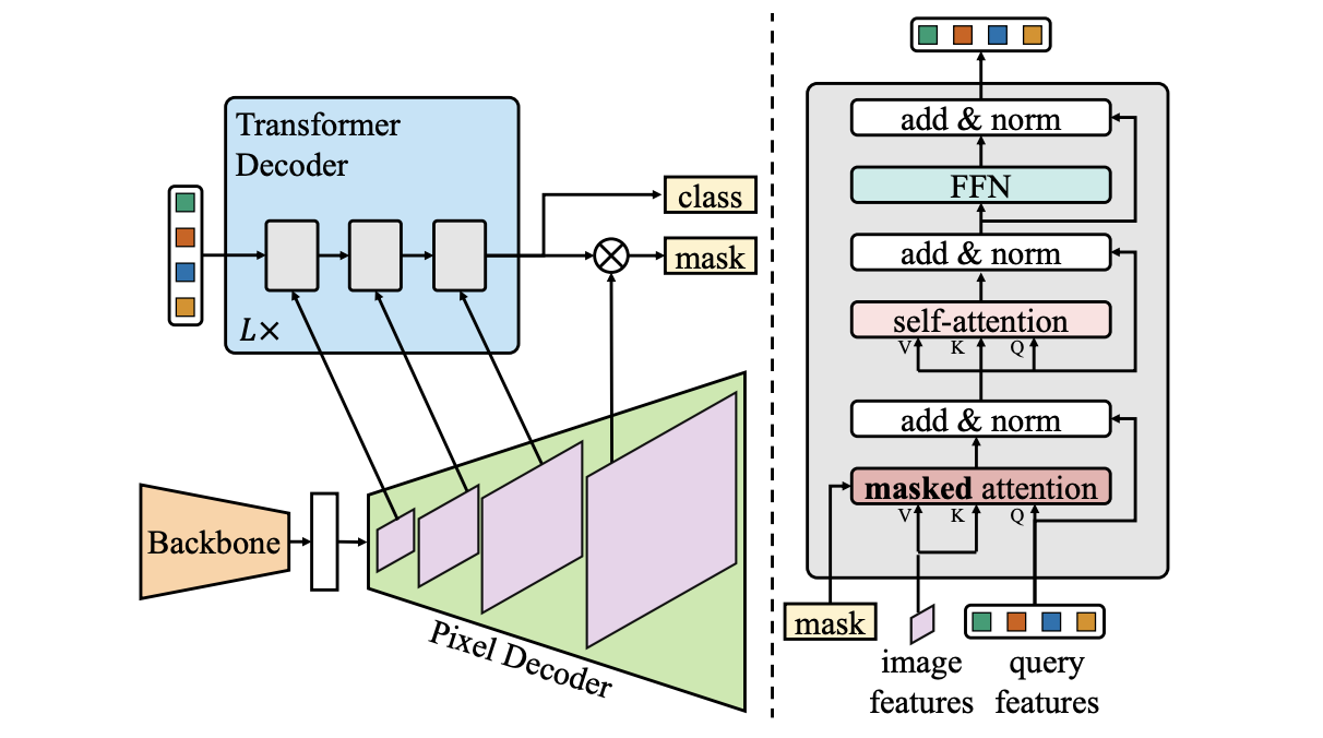
Masked attention:
-
Idea: constrain attention only to the foreground area corresponding to the query.
-
Standard self-attention:
-
Masked attention:
Mask2Former: Summary
-
Note that we do not talk about "stuff" and "things" anymore.
-
Queries abstract those notions away.
-
Achieves state-of-the-art accuracy across segmentation tasks.
Conclusions
-
Transformers have revolutionized the field of NLP, achieving incredible results.
-
We observe massive impact on computer vision(DETR, ViT).
-
Complementing CNNs, Transformers have reached state-of-the-art in object classification, detection, tracking, and image generation.
-
A grain of salt: This often comes at an increased computational budget(larger GPUs, longer training).
Unsupervised
Learning without labels
Compact, yet descriptive representation?
Consider the loss:
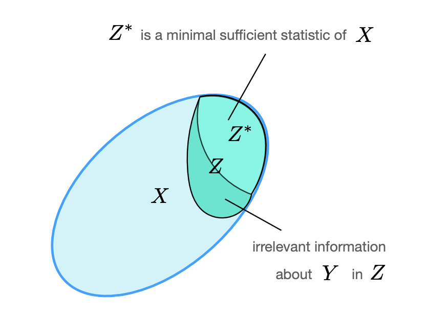
where
-
: Minimize MI between and (compression).
-
: Preserve relevant information in about .
Recap: Mutual Information(MI)
After obtaining compact and descriptive representation, we can apply it for different tasks, such as detection, classification, segmentation, etc. by adding task-specific shallow models(e.g., linear projection).
Evaluating Self-supervised learning(SSL) models
-
Fine-tuning on the downstream tasks:
-
Either all or only few last layers.
-
Pros: Typically leads to best task performance(e.g., accuracy, IoU).
-
Cons: Our model becomes task-specific; cannot be re-used for other tasks.
-
-
Linear probing:
-
Only learn the new linear projection. The model parameters remain fixed.
-
Pros: We can re-us the model for other tasks by training multiple linear projections.
-
Cons: Typically worse task accuracy than fine-tuning.
-
-
k-NN classification:
-
Project labeled data in the embedding space.
-
Classify datapoints according to the class of its k nearest neighbors.
-
Pros: Same as linear probing(versatility), but no learning is necessary.
-
Cons: Prediction can be a bit costly.
- Linear search complexity due to high feature dimensionality.
-
-
How do we train deep models without labels?
-
Goal: Define training objectives with some relation to our target objective.
-
By training the model on these objectives, we hope to learn something for the target objective.
-
-
Categories of self-supervision
-
Pretext tasks
-
Contrastive learning
-
Non-contrastive learning
-
Pretext tasks
Idea: Solve a different task with available(generated) supervision.
Caveats:
-
The task should have some relation to our goal task.
-
Finding an effective pretext task is challenging.
-
The deep net will always try to cheat, i.e. find "shortcut" solutions.
Pretext task: Rotation
Task: predicting image rotation.
Training process outline
-
Quantize rotation angles(e.g., 0, 90, 180, 270 - 4 classes).
-
Sample an image from the training dataset.
-
Rotate the image by one of the pre-defined angles.
- This defines our "ground-truth" label.
-
Train the network to predict the correct rotation class.
-
This leverages the photographic bias in typical image datasets
- i.e. photographed objects have prevalent orientation.
-
Otherwise, there’s no canonical pose, hence the rotation angles are meaningless.
- A thought experiment: add all rotated images to the original dataset.
Pretext task: Jigsaw puzzle
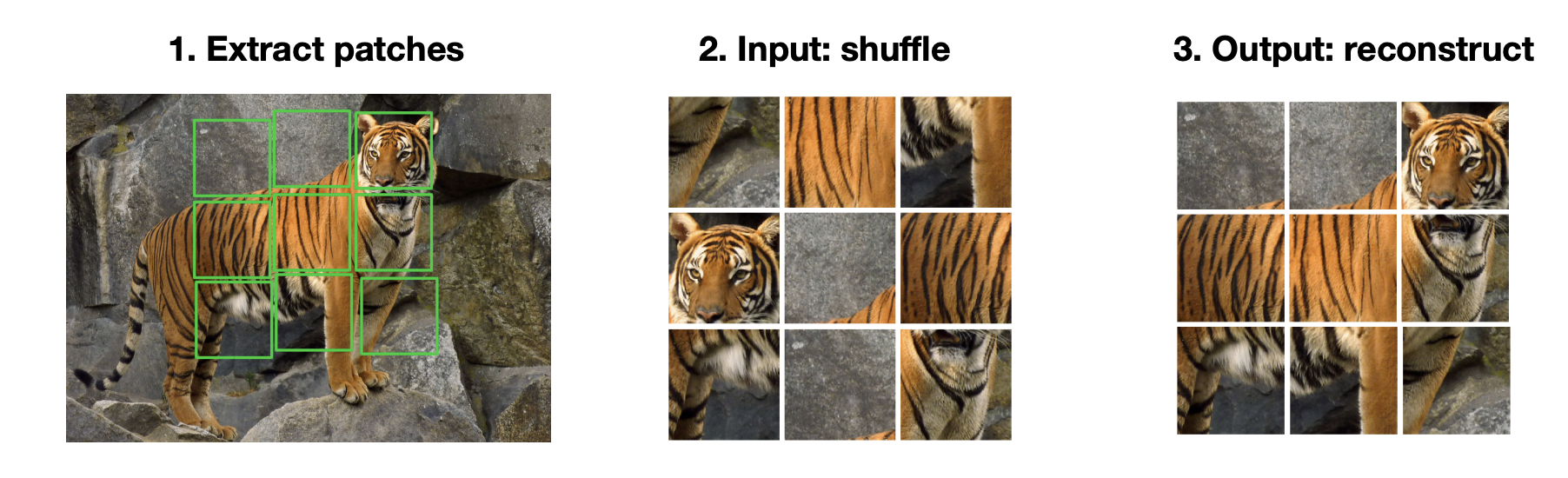
-
Solving this task requires the model to learn spatial relation of image patches.
-
Cast this task as a classification problem:
- Every permutation defines a class.
Pretext task: Colorization
Predicting the original color of the images(in CIELAB color space):
Intuition: Proper colorization requires semantic understanding of the image.
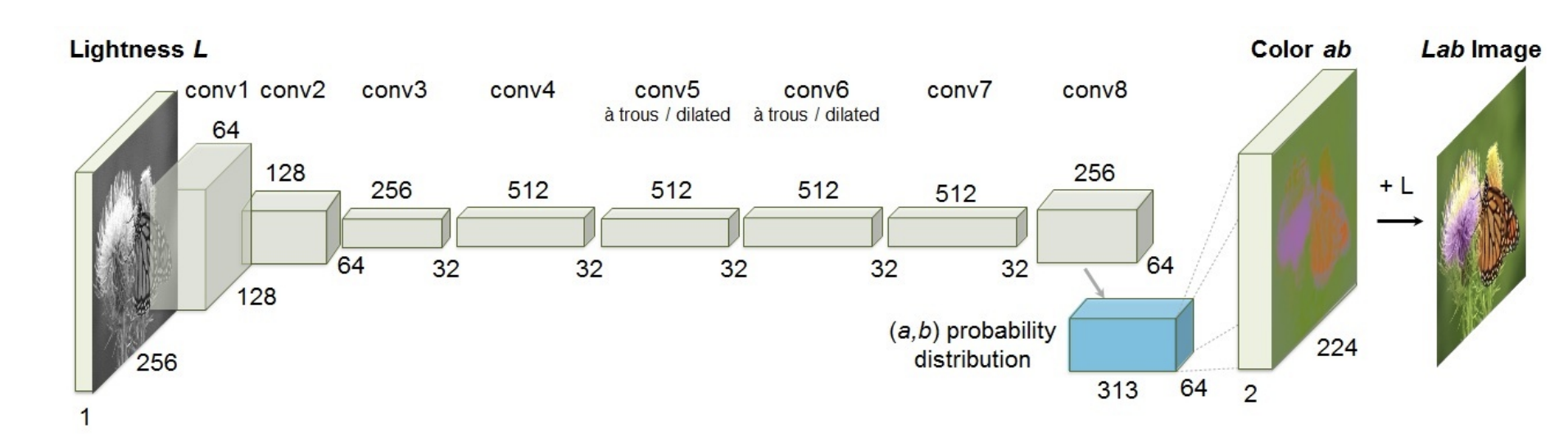
Nuances:
-
This is not the same as predicting RGB values from a greyscale image(due to multimodality of colorization).
-
Instead, we operate in Lab color space. Recall:
-
L stands for perceptual lightness;
-
a and b express four unique colors(red, green, blue, yellow).
-
-
Euclidean distances in Lab are more perceptually meaningful.
-
We cast colorization as a multinomial classification problem.
-
Example: Colorization of black-and-white photos.
Contrastive learning
Recall metric learning
Intuitive idea:

We need labels to define positive and negative pairs.
Contrastive learning is an extension of metric learning to unsupervised scenarios.
Idea:
-
Use data augmentation(e.g., cropping) to create a positive pair of the same image.
-
Use other images to create(many) negative pairs.
Example:
-
Represent each image as a single feature vector(e.g., last layer in a CNN).
-
Consider cosine similarity of two such vectors:
-
For a given set compute contrastive score.
-
Temperature : a hyperparameter(usually between 0.01 and 1.0).
-
What is the range?
-
What does it mean when it reaches maximum/minimum?
-
We clearly want to maximize this value!(many implementations)
-
Example loss: .
-
Intuition
-
Note that we normalize the feature embeddings:
-
Every unit vector corresponds to a point on a unit sphere.
-
The goal of contrastive learning is to cluster the representation on the sphere.
-
The points on the sphere will be linearly separable.
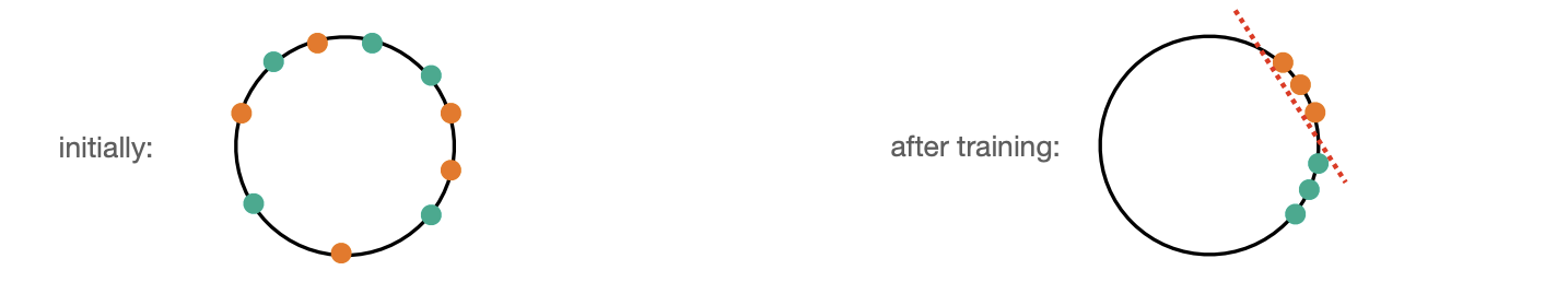
Intuition
Deep frameworks for SSL
-
SimCLR
- A simple framework for contrastive learning.
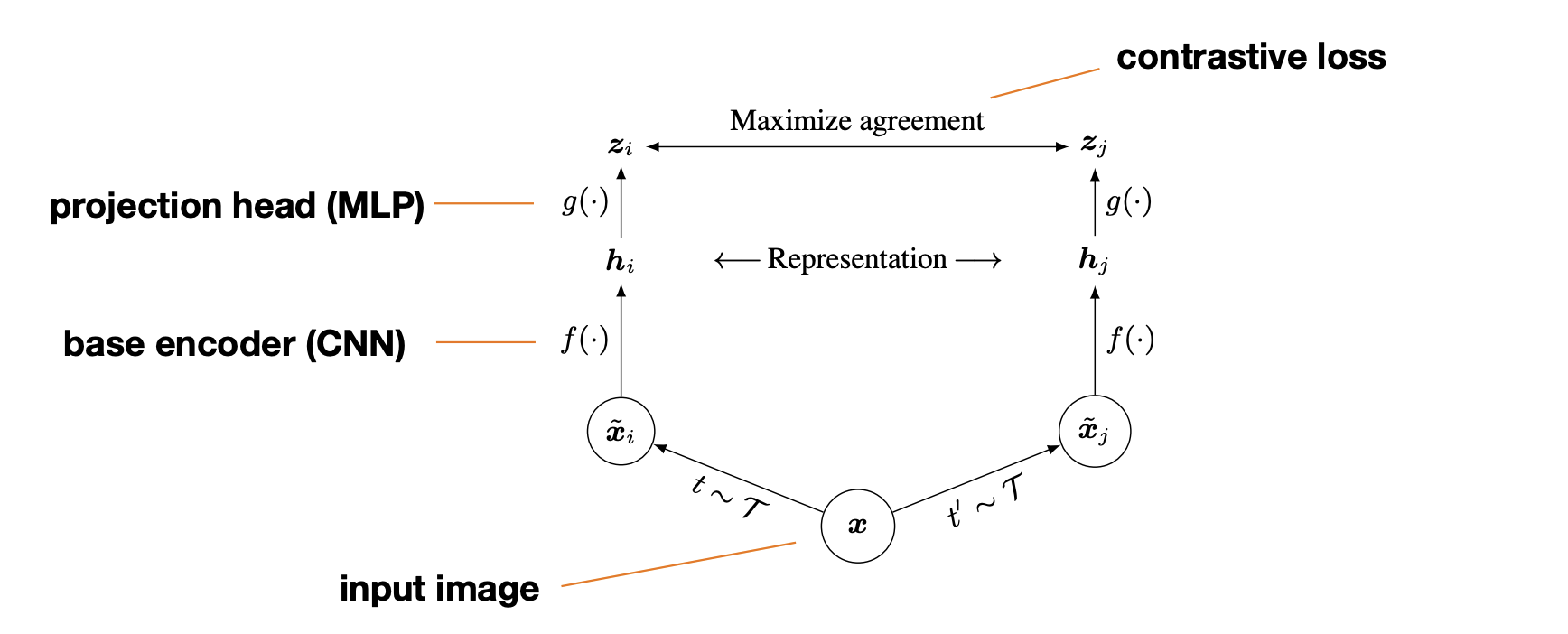
SimCLR -
Conceptually very simple.
-
Best results require substantial computational resources
- batch size 8192(16382 negative pairs)
-
Why do we need a large batch size?
- A subject of ongoing research. - Intuition: More negative samples reduce the gradient variance.
-
-
BYOL
-
MoCo
- Reduced the GPU memory footprint by applying momentum encoder:
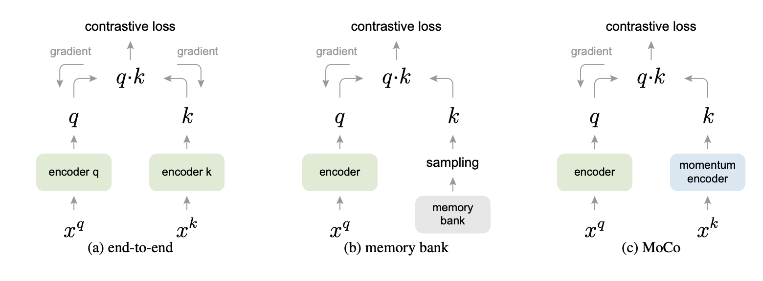
Momentum encoder 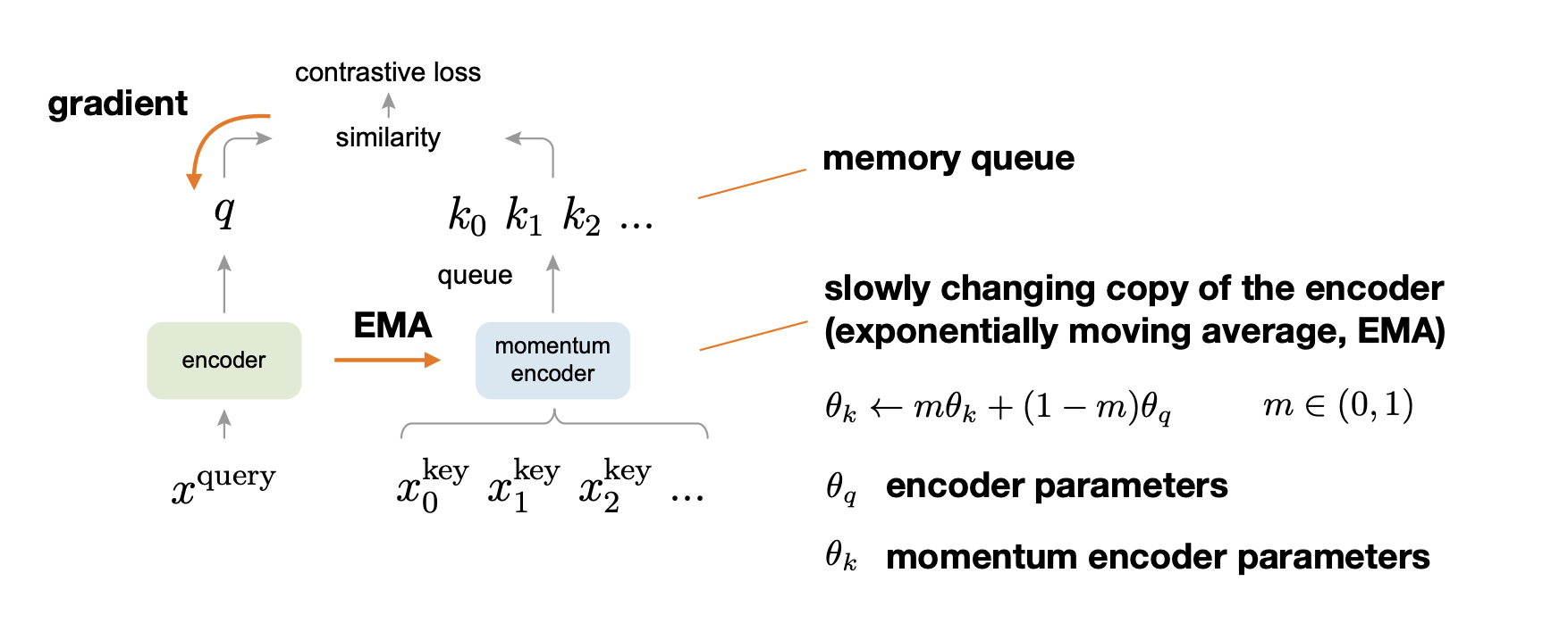
MoCo -
DINO
-
Masked Autoencoders
-
and many more…
Non-contrastive learning
DINO
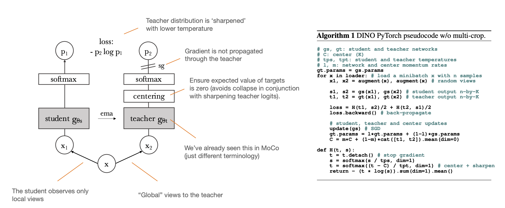
-
Simple to implement and to train.
-
Broad application spectrum.
-
Self-distillation with no labels.
-
Self-attention maps in the last layer of a ViT with respect to [CLS] token.
-
Different heads also focus on semantically distinguishable features.
-
The attention maps are temporally stable.
DINOv2
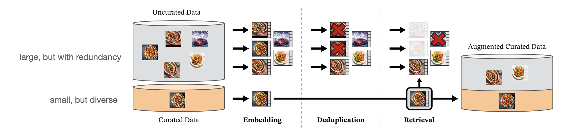
-
X2 faster and X3 less memory than DINO.
-
A combination of existing techniques(e.g. noisy student, adaptive resolution).
-
Training one big model, distilling to the smaller networks.
-
Careful data curation.
Masked Autoencoders
Unsupervised learning with Transformers and a reconstruction loss:
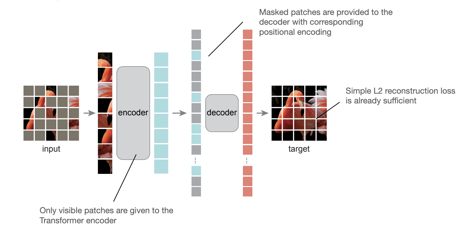
Reconstructing HoG features, instead of pixel values:
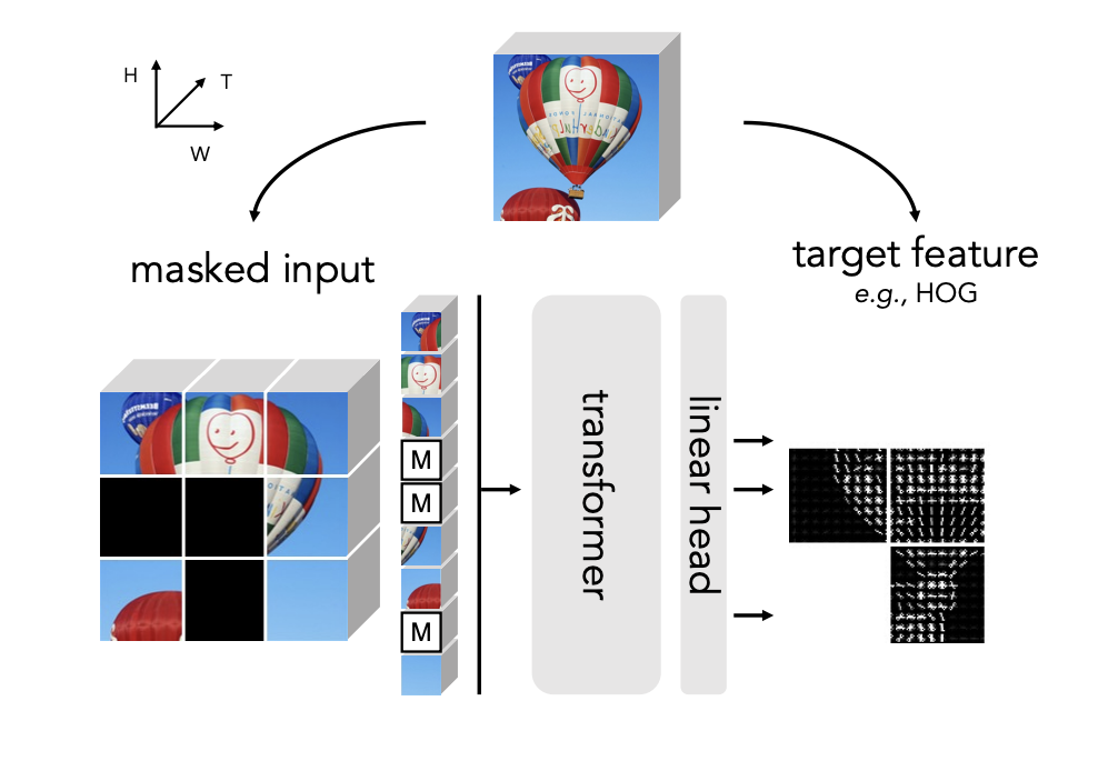
Remarks:
-
High masking ratio is necessary(75% or more).
-
Compute the loss only on the patches masked out in the input:
- This is different from denoising autoencoders.
-
Reconstruction w.r.t. normalized values:
- compute the mean and deviation of pixels within each patch.
-
Why does this work:
- This behavior occurs by way of a rich hidden representation inside the MAE.
- Intuition: The goal is not much different from contrastive learning!
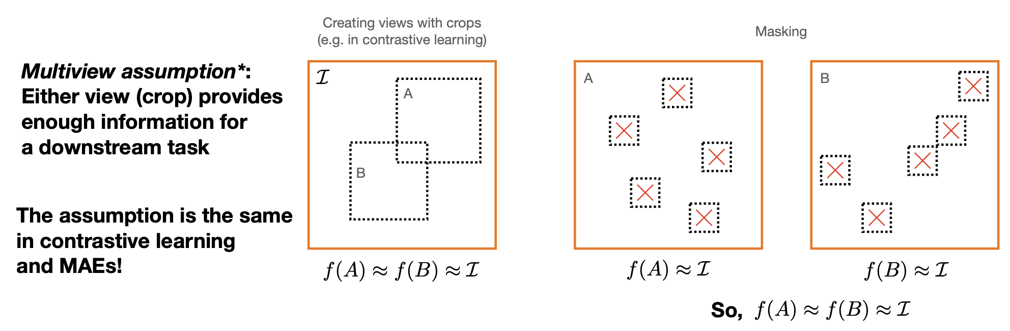
Multi-view assumption
Downstream applications
What do DINO features encode?
DINO(and other SSL methods) provides semantic correspondence(almost) out-of-the-box.
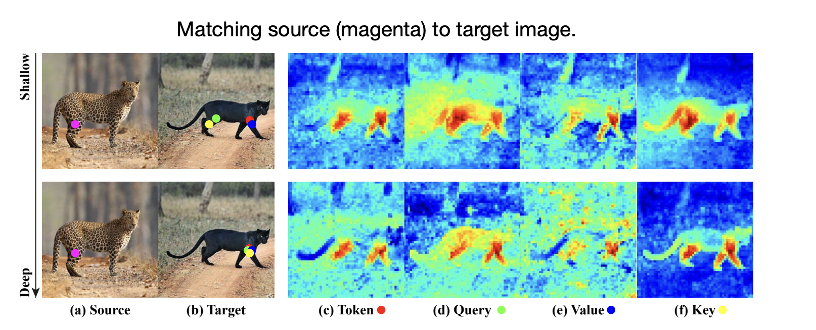
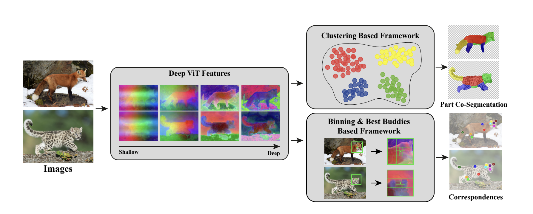
We can also cluster "background" (stuff) areas, hence obtain semantic segmentation.
High level idea: Learn a lower dimensional embedding, , such that clustering in this space yields semantic masks.
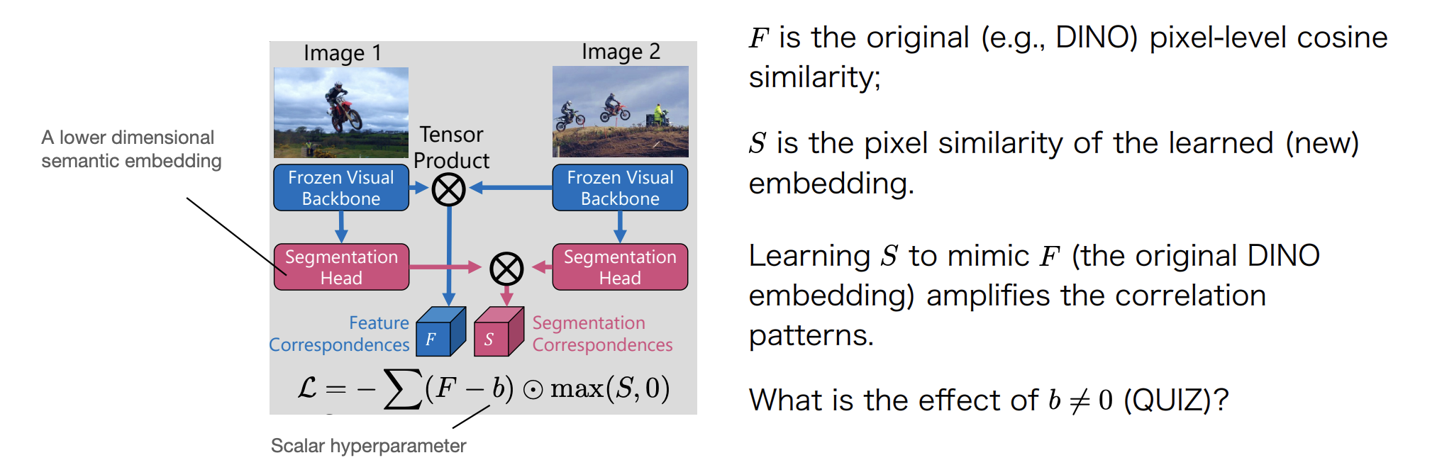
Self-supervision in videos
Two groups of problems:
-
Given a video, segment objects in the video(using motion cues).
-
Given a video dataset, learn to track objects.
Segmentation from motion cues Idea: If the object mask is correct, we cannot reconstruct object-related optical flow. We train two networks
-
Network G: Given an image and optical flow, predict object mask (foreground/background).
-
Network I: Given a masked optical ow and the image (not masked), reconstruct the original optical flow.
Contrastive random walk
Forward-backward cycle consistency:
-
Given a video, construct a palindrome(i.e. )
-
Label each patch in the image and propagate them through a video.
- We compute affinity(using cosine similarity) between patches of subsequent frames.
-
Cycle consistency loss: Each label should arrive at its original location.
Conclusion
-
Research on unsupervised learning is very active.
-
We can train more accurate models with less supervision.
-
Requires large computational resources(dozens of high-end GPUs).
-
Yet do not scale(too) well with the amount of data(saturation).
-
Many open questions:
-
What is a good proxy task?
-
How to make computational requirements manageable?
-
How (and/or why) does it work?
-
Semi-supervised learning
Training on labeled and unlabeled data.
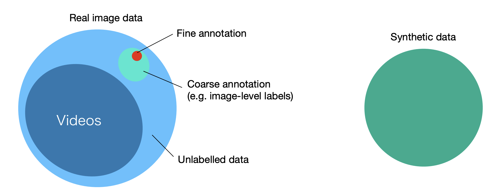
General remarks:
-
Using both labeled and unlabeled data is a very practical scenario.
-
If the goal is to get the best accuracy, semi-supervised learning is the way to go.
- Current state-of-the-art frameworks take this approach(rather than full supervision).
Small print:
-
Improvement is not always guaranteed.
- It depends on the model, the technique used and the unlabeled data.
-
Semi-supervised techniques are often complementary.
- A combination of multiple techniques yields the best results(though make the framework more complex).
A practical perspective:
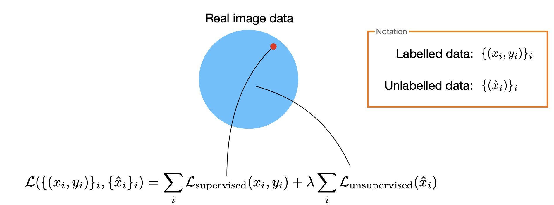
Assumptions
Assumptions about semi-supervised learning:
Smoothness assumption
If two input points are close by, their labels should be the same.
Transitivity
-
We have a labeled and two unlabeled inputs.
-
Suppose is close to , and is close to , but is not close to .
-
Then we can still expect to have the same label as .
Low-density assumption
The decision boundary should pass through a region with low density .
Manifold assumption
-
Data comes from multiple low-dimensional manifolds.
-
Data points sharing the same manifold, share the same label.
Remark:
Which assumptions to make depends on what we know about how our data distribution interacts with the class posterior .
Two taxonomies
How unlabeled data is used:
Unsupervised pre-processing
- pre-training, clustering, etc.;
- Two stages:
-
Unsupervised: Feature extraction/learning(e.g. DINO, MAE).
-
Supervised: Fine-tuning, linear probing, or k-NN classification.
Wrapper methods
Self-training
A single classifier trained jointly on labeled and self-labeled data from the unlabeled dataset.
OnAVOS:
Online adaptation: Adapt model to appearance changes in every frame, not just the first frame.
Drawback: Can be slow.
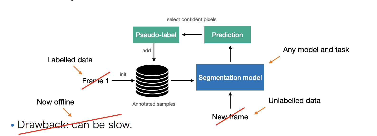
Segment Anything (2)
Self training with pseudo labels
-
How to select pseudo-labels(the confidence threshold)?
-
High vs. low threshold trade-off(QUIZ)
-
High: No learning signal(the gradient will be close to zero);
-
Low: Noisy labels low accuracy
-
-
Tedious to train(Multiple training rounds).
-
Sensitive to the initial model:
- Fails if the initial predictions are largely inaccurate.
A general outline:
-
Train a strong baseline on the labeled set;
- e.g. with heavy data augmentation(crops, photometric noise).
-
Predict pseudo-labels for the unlabeled set.
-
Continue training the network on both labeled and pseudo-labeled samples.
-
Repeat steps 2-3.
Intrinsically semi-supervised
Entropy minimization
-
Example:
Entropy minimization for semantic segmentation("self-training"):
-
Objective:
Minimize the entropy of class distribution for each pixel:
Virtual adversarial network
Idea: Perturbations of the input should not change the label.
-
supervised case. We want to minimize:
where
-
Semi-supervised case:
Replace above with our current estimate,
Learning from synthetic data
Labeled and unlabeled data may come from different distributions.
e.g. due to differences in the synthetic and real appearances.
-
Labels are easier(hence cheaper) to obtain on a large scale.
-
Consider it a special case of a semi-supervised learning problem.
Domain alignment
This translates into disjoint feature distribution of a model trained only on the labeled data:
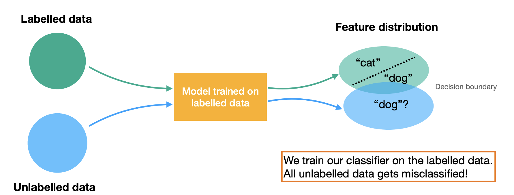
Solution: "Align" the two distributions.
Domain alignment means making two feature distributions indistinguishable.
We can use a GAN:
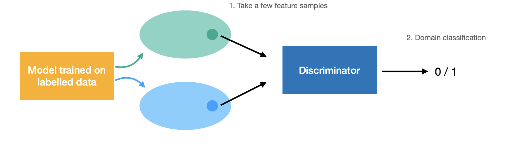
-
The discriminator learns to classify the origin of the provided feature.
-
The model learns:
-
to classify the labeled images.
-
a feature representation that reduced discriminator accuracy.
-
Consistency regularization
Consistent prediction across image transformations.
Semantic meaning does not change, though not guaranteed in a deep net Use it as a consistency loss.
Framework:
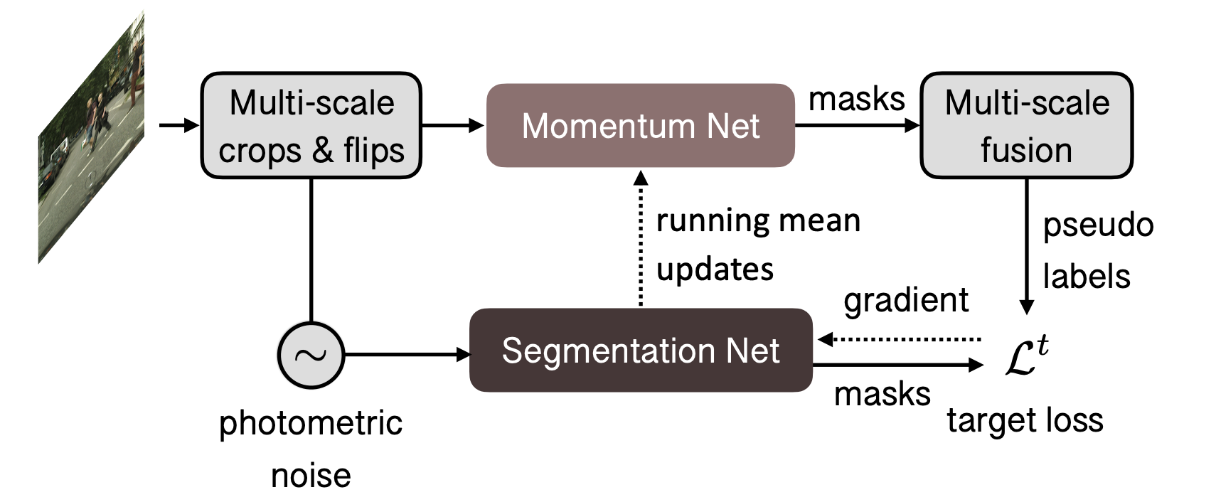
Momentum net
Test-time augmentation is applied online at training time:
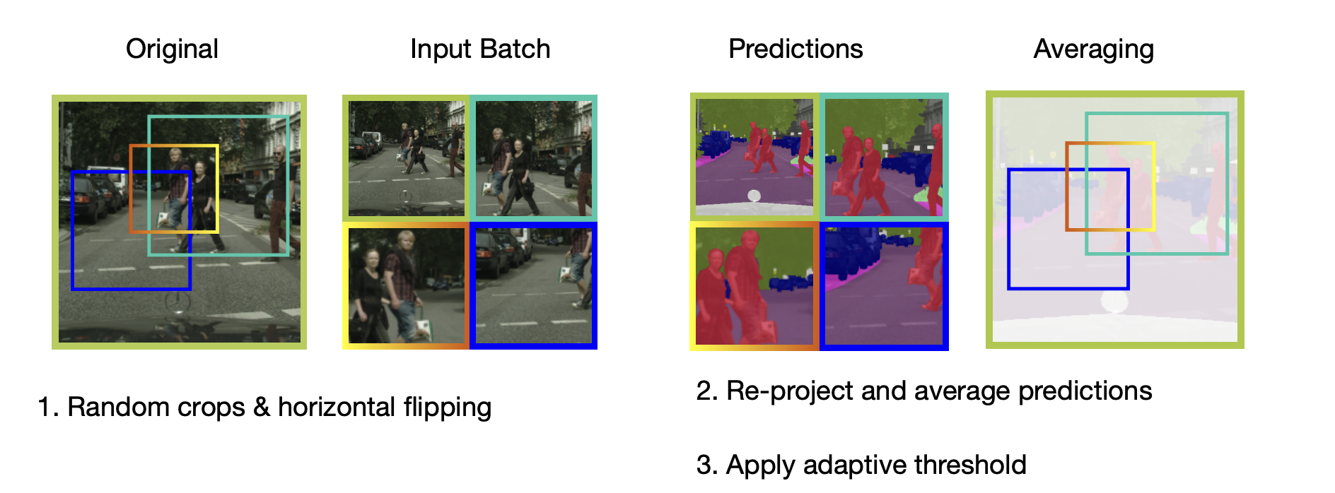
Limited supervision
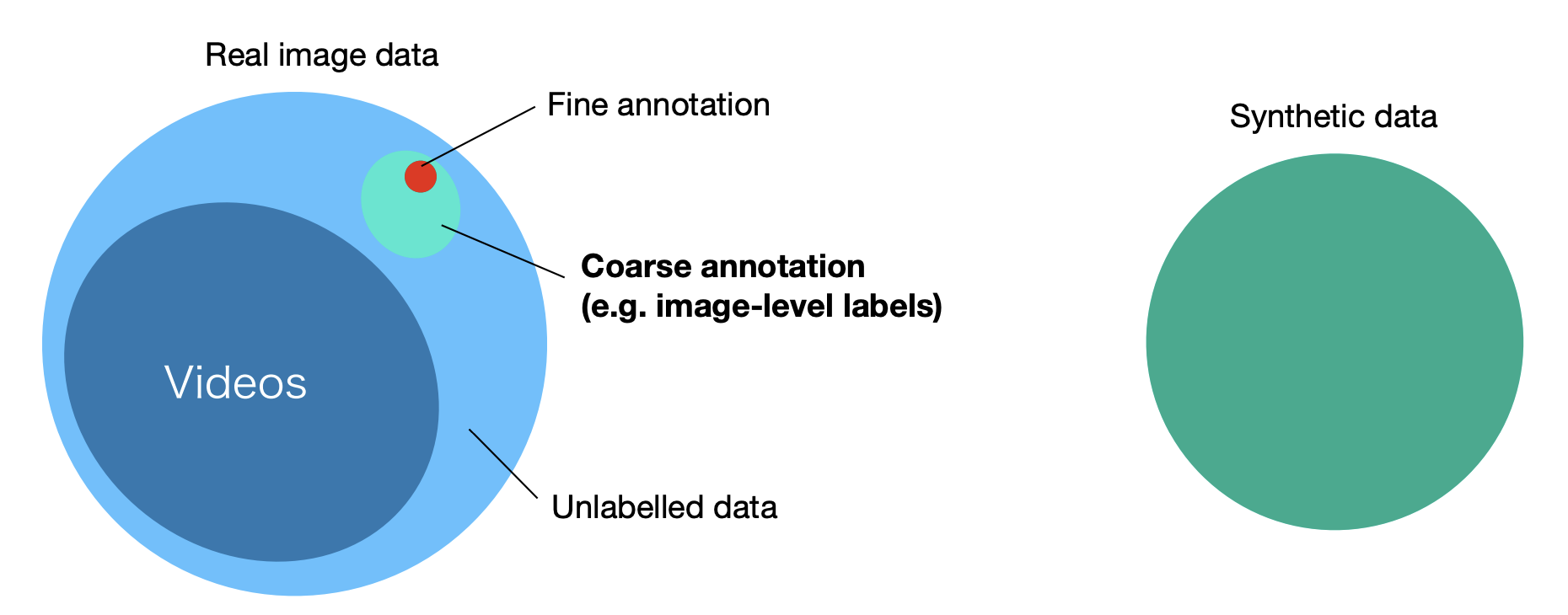
Weakly supervised learning: training coarse labels:
Segmentation with image-level labels
Idea: we can reuse the classifier weights to classify every pixel.
-
Consider a classification network:
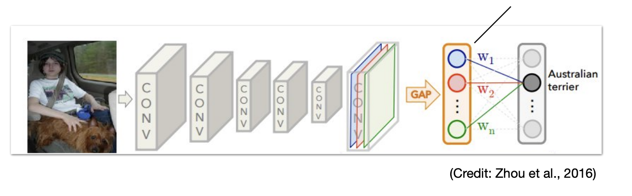
Classification network -
We can replace GAP and instead use convolution.
-
Insight: such classification turns out to be meaningful.
Summary
-
Entropy minimization
- Improves accuracy, but leads to miscalibration.
-
Virtual adversarial network
- generic treatment of supervised and unsupervised data.
-
Consistency regularization
- can be effective, but sensitive to initial pseudo-label quality.
-
Self-training
- simple and effective; but is limited by available augmentation techniques.
-
Unsupervised pre-training
- simple and effective; this should be your first baseline.
-
Domain alignment
- typically less fine-tuning is required, but can be still challenging to train(GAN).
-
Coarse labels(weak supervision)
- a cost-effective compromise between fully labeled and unlabeled data.

Introduction and Object Detection
What this course is
Hight-level(semantic) computer vision:
-
Object detection
-
image segmentation
-
object tracking
-
etc...
From another perspective this is the intersection of Computer vision, deep learning and real-world applications, as shown in Fig 1.
What is computer vision:
-
First defined in the 60s(The summer vision project 1966).
-
"Mimic the human visual system.
-
Center block of artificial intelligence.
Semantic scene understanding:
-
Classification
-
Object detection
-
Semantic segmentation
-
Instance segmentation
-
Object tracking
This course in two dimension is as shown in Fig 2.
Understanding an image
Different representations depending on the granularity
-
Detection (bounding box-coarse description)
-
Semantic segmentation(pixel-level)
-
Instance segmentation(e.g. "person 1", "person 2")
Understanding a video
Why use the temporal domain
-
Motion analysis, multi-view reasoning.
-
A smoothness assumption: no abrupt changes between frames.
But challenges:
-
High computational demand.
-
A lot of redundancy.
-
Occlusions, multiple objects moving and interacting.
Some architectures and concepts
-
R-CNN, Fast R-CNN and Faster R-CNN (2-stage object detection)
-
YOLO, SSD, RetinaNet (1-stage object detection)
-
Siamese networks (online tracking)
-
Message Passing Networks (offline tracking)
-
Mask R-CNN, UPSNet (panoptic segmentation)
-
Deformable/atrous convolutions
-
Graph neural networks(GNNs)
-
Vision Transformers(ViT), DETR(object detection), SAM
-
Contrastive learning
Object detection
One-stage detectors
One-stage detectors treat object detection as a single task, directly predicting the object class and bounding box coordinates from the input images.
Object detection with sliding window
For every position, measure the distance(or correlation) between the template and the image region(See Fig 3):
where is the distance metric, is the image
region, and is the template.
Template matching distances
-
Sum of squared distances(SSD), or mean squared error(MSE):
-
Normalized cross-correlation(NCC):
-
Zero-normalized cross-correlation(ZNCC):
Disadvantages
-
(Self-) Occlusions
- e.g. due to pose changes
-
Changes in appearance
-
Unknown position, scale, and aspect ratio
- brute-force search(inefficient)
Feature-based detection
Idea: Learn feature-based classifiers invariant to natural object changes(See Fig 4)
-
Features are not always linearly separable
-
Learning multiple weak learners to build a strong classifier(Fig 5)
Multiple weak learners
Viola-Jones detector
Given data
-
Define a set of Haar-like features(Fig 6)
Haar-features are sensitive to directionality of patterns
Haar features -
Find a weak classifier with the lowest error across the dataset
-
Save the weak classifier and update the priority of the data samples
-
Repeat Steps 2-3 times
Final classifier is the linear combination of all weak learners.
Histogram of Oriented Gradients
Average gradient image over training samples gradients provide shape information.
HOG descriptor Histogram of oriented gradients.
Compute gradients in dense grids, compute gradients and create a histogram based on gradient direction.
-
Choose your training set of images that contain the object you want to detect.
-
Choose a set of images that do NOT contain that object.
-
Extract HOG features from both sets.
-
Train an SVM classifier on the two sets to detect whether a feature vector represents the object of interest or not(0/1 classification)
Deformable Part Model
Many objects are not rigid, so we could use a Bottom-up approach:
-
detect body parts
-
detect "person" if the body parts are in correct arrangement
Note: The amount of work for each RoI may grow significantly.
Two-stage detectors
Two-stage object detectors split the object detection task to two parts(Fig 7):
-
Region Proposal: The network first identifies potential regions in the image that may contain objects.
-
Refinement: These regions are further analyzed to classify the objects and refine their bounding boxes.
A generic, class-agnostic objectness measure: object proposals or regions of interest(RoI)
Object proposal methods:
-
Selective search
- Using class-agnostic segmentation at multiple scales.
-
Edge boxes
- Bounding boxes that wholly enclose detected contours.
Non-Maximum Suppression(NSM)
Method to keep only the best proposals(See algorithm [alg:nms]).
Region overlap
We measure region overlap with the Intersection over Union(IoU) or Jaccard Index:
The threshold is the decision boundary used to determine whether a detected object or prediction should be considered valid. For example, in object detection:
-
Choosing a high threshold ‒ more false positives, low precision
-
Choosing a low threshold ‒ more false negatives, low recall
Object detection with deep networks
Overfeat
Explores three well-known vision tasks using a single framework.
-
Classification
-
Localization
-
Detection
Training convolution on all tasks boosts up the accuracy, see Fig 8.
Apply Non-Max Suppression to combine the predictions and windows, see Fig 9.
Improved detection accuracy is largely due to feature representation learned with deep nets.
But cons:
-
Expensive to try all possible positions, scales and aspect ratios.
-
The network operates on a fixed resolution.
The complexity of a sliding window is , where is the number of all the windows, and represents the amount of work needed to perform detection and classification for one window. The complexity of the "pre-filtered" method is , where is the amount of work needed for filtering each window, and is the number of windows left after being filtered.
"Pre-filtering" method pays off when:
Assume the constant factors are comparable/negligible:
where is the Region-of-Interest(RoI) ratio, and is the efficiency of RoI generator. In practice, there is a delicate balance between and : Reducing and increasing .
Object proposals(Pre-filtering) and pooling for two-stage detection
Heuristic-based object proposal methods:
-
Selective search
- Using class-agnostic segmentation at multiple scales.
-
Edge boxes
- Bounding boxes that wholly detected contours
R-CNN family(Regions with CNN features)
-
Spatial Pyramid Pooling(SPP)
-
(Fast/Faster) R-CNN
-
Region Proposal Network(RPN)
R-CNN
Training scheme:
-
Pre-train the CNN for image classification(ImageNet)
-
Finetune the CNN on the number of classes the detector is aiming to classify
-
Train a linear SVM classifier to classify image regions - one linear SVM per class
-
Train the bounding box regressor
Pros:
-
New: CNN features; the overall pipeline with proposals is heavily engineered – Good accuracy.
-
CNN summarizes each proposal into vector.
-
Leverage transfer learning: The CNN can be pre-trained for image classification with c classes. One needs only to change the FC layers to deal with Z classes.
Cons:
-
Slow: 47s/image with VGG 16 backbone. One considers around 2000 proposals per image, they need to be warped and forwarded through the CNN.
-
Training is also slow and complex.
-
The object proposal algorithm is fixed.
-
Feature extraction and SVM classifier are trained separately - features are not learned "end-to-end".
Problems:
-
Input image has a fixed size
FC layer prevents us from dealing with any image size.
-
TBD
Fast R-CNN
Fast R-CNN = R-CNN + RoI Pooling(Single layer SPP-Net)
RoI Pooling RoI Pooling is a technique introduced in the Fast R-CNN framework to efficiently extract fixed-size feature representations for arbitrary regions(bounding boxes) in a feature map. It address the problem of feeding region proposals of various sizes into a neural network in a way that:
-
Preserves spatial information with each region of interest(RoI).
-
Produces a fixed-dimensional feature vector needed by fully connected layers(classifiers).
1. Feature extraction for the entire image
Instead of cropping individual region proposals from the original image and passing them each though a ConvNet(as done in older approaches like R-CNN), we:
-
Feed the entire image into a convolutional neural network(e.g., VGG, ResNet).
-
Obtain the resulting feature map, typically a 2D grid of activations.
This means the network only processes the image once, which is much more efficient.
2. Mapping region proposals to the feature map
You have a set of region proposals(bounding boxes) in the original image coordinates-these come from an external region proposal method(e.g., selective search) or from a region proposal network(in Faster R-CNN).
Each region proposal is then mapped onto the feature map coordinates:
- Because the CNN reduces spatial resolution(due to pooling layers or strided convolutions), the coordinates of each region of the original image need to be scaled to align with the coordinate system of the smaller feature map.
3. Dividing each RoI into Sub-regions
To handle different RoI sizes but produce a fixed-size output(for example 7X7 output grid in Fast R-CNN):
-
Divide the mapped RoI on the feature map into a predefined grid(e.g., 7X7).
-
Each sub-region in this grid corresponds to a smaller set of feature map cells.
4. Pooling operation
Within each of these sub-regions(bins):
-
Perform a pooling operation(usually max pooling, though average pooling can also be used).
-
This operation collapses the variable-sized sub-region into a single value(e.g., the maximum activation within that bin).
By doing this for each subregion in the grid, you transform the entire RoI into a fixed-size feature map(e.g., 7X7), regardless of the original size of the bounding box.
5. Feeding pooled features to classifier layers
Note that you have a fixed spatial dimension(e.g., 7X7), you can:
-
Flatten or otherwise reshape this pooled feature map.
-
Pass it into fully connected layers(and ultimately classification/regression heads) to predict:
- The object class for that region.
- The bounding box refinement offsets, etc.
Result of Fast R-CNN
Faster R-CNN
Faster R-CNN = Fast R-CNN + Region proposal network
Region Proposal Network: We fix the number of proposals by using a set of anchors per location.
A 256-d descriptor characterizes every location.
For feature map location, we get a set of anchor corrections and classification into object/non-object.
RPN: Training
Classification ground truth: We compute which indicates how much an anchor overlaps with the ground truth bounding boxes:
-
1 indicates that the anchor represents an object(foreground), and 0 indicates a background object. The rest do not contribute to the training.
-
For an image, randomly sample a few(e.g., 256) anchors to form a mini-batch(balanced objects vs. non-objects)
-
We learn anchor activate with the binary cross-entropy loss
-
Those anchors that contain an object are used to compute the regression loss.
-
Each anchor is described by the center position, width and height().
-
What the network actually predicts are:
\[\begin{equation} t_x = \frac{x - x_a}{w_a}
\end{equation}]
\[\begin{equation} t_y = \frac{y - y_a}{h_a}
\end{equation}]
\[\begin{equation} t_w = \log\!\biggl(\frac{w}{w_a}\biggr)
\end{equation}]
\[\begin{equation} t_h = \log\!\biggl(\frac{h}{h_a}\biggr)
\end{equation}]
-
Smooth L1 loss on regression targets
Faster R-CNN training:
- First implementation, training of RPN separate from the rest.
- Now we can train jointly!
- Four losses:
-
RPN classification(object/non-object)
-
RPN regression(anchor – proposal)
-
Fast R-CNN classification(type of object)
-
Fast R-CNN regression(proposal – box)
Feature Pyramid Networks
CNNs are not scale-invariant.
-
Idea A: Featurised image hierarchy
Featurised image hierarchy - Pros: Typically boosts accuracy(esp. at test time).
- Cons: Computationally inefficient.
-
Idea B: Pyramidal feature hierarchy
Pyramidal feature hierarchy - More efficient than Idea A, but
- Limited accuracy(inhibits the learning of deep representations)
-
Feature pyramid network(FPN)
Feature pyramid network - Higher scales benefit from deeper representation from lower scales.
- Efficient and high accuracy.
Straightforward implementation:
-
Convolution with 1 X 1 kernel
-
Upsampling(nearest neighbours)
-
Element-wise addition
Integration with RPN for object detection:
-
Define RPN on each level of the pyramid.
-
Only a single-scale anchor per level(scale varies across levels).
-
At test time, merge the predictions from all levels.
Pros:
-
Improves recall across all scales(esp. small objects).
-
More accurate(in terms of AP).
-
Broadly applicable, also for one-stage detectors.
-
Still in wide use today.
Cons: Increased model complexity.
Single-stage object detection
YOLO
-
Define a coarse grid().
-
Associate B anchors to each cell.
-
Each anchor is defined by:
- Localization(x, y, w, h).
- A confidence value(object/no object).
- And a class distribution over C classes.
Inference time:
It is more efficient than Faster R-CNN, but less accurate.
-
Coarse grid resolution, few anchors per cell = issues with small objects
-
Less robust to scale variation.
SSD
Pros:
-
More accurate than YOLO.
-
Works well even with lower resolution improved inference speed.
Cons:
-
Still lags behind two-stage detectors.
data augmentation is still crucial(esp. random sampling).
-
A bit more complex(due to multi-scale features).
RetinaNet
Problems with one-stage detectors
Two-stage detectors:
-
Classification only works on "interesting" foreground regions(proposals, 1-2k). Most background examples are already filtered out.
-
Class balance between foreground and background objects is manageable.
-
Classifier can concentrate on analyzing proposals with rich information.
Problems with one-stage detectors:
-
Many locations need to be analyzed(100k) densely covering the image - foreground-background imbalance.
- Many negative examples(every cell on the feature grid).
- Few positive examples(actual number of objects).
-
Hard negative mining: subsample the negatives with the largest error:
- works, but can be unstable.
Class imbalance:
- Idea: balance the positives/negatives in the loss function.
- Recall cross-entropy loss:
Focal loss
Replace CE with focal loss(FL):
-
When , it is equivalent to the cross-entropy loss.
-
As goes towards 1, the easy examples are down-weighted.
-
Example: , if , FL is lower than CE.
RetinaNet
-
One-stage(like YOLO and SSD) with Focal Loss.
-
Feature extraction with ResNet.
-
Multi-scale prediction - now with FPN.
Spatial Transformers
Features of Spatial pooling:
-
Helps detect the presence of features.
-
No information about precise location of features within a RoI.
- No effect on the RoI localization.
Solution: Spatial Transformers.
Equivariance is needed:
-
Learn to predict the parameters of the mapping :
Spatial Transformers -
Learn to predict a chain of transformations.
-
Learn to localize RoI without dense supervision(only class label).
-
Training multiple STs: Focus on different object parts.
-
Learning to localize without any supervision.
-
Makes the network equivariant to certain transformers(e.g., affine).
-
Fully differentiable.
Cons:
- Difficulty of training for generalizing to more challenging scenes.
Detection evaluation
Precision: How many zebras you found are actually zebras?
Recall: How many actual zebras in the image/dataset you could find?
What is a true positive?
-
Use the Intersection over Union(IoU).
-
e.g., if – positive match
-
The criterion is defined by the benchmarks(MS-COCO, Pascal VOC)
Resolving conflicts
-
Each prediction can match at most 1 ground truth box.
-
Each ground truth box can match at most 1 prediction.
All-in-one metric: Average precision(AP)
There is often a trade-off between Precision and Recall.
AP = the area under the Precision-Recall curve(AUC)
Computing average precision
-
Sort the predicted boxes by confidence score
-
For each prediction find the associated ground truth
- The ground truth should be unassigned and pass IoU threshold
-
Compute cumulative TP and FP:
- TP: [1, 0, 1] FP: [0, 1, 0] cTP = [1, 1, 2], cFP = [0, 1, 1]
-
Compute precision and recall(#GT = 3 TP + FN + 3)
- Precision: ; Recall(#GT=3):
-
Plot the precision-recall curve and the area beneath(num. integration).
mAP is the average over object categories
Single object tracking
Problem statement: Given observations at , and find their correspondence at
Challenges:
-
Fast motion.
-
Changing appearance.
-
Changing object pose.
-
Dynamic background.
-
Occlusions.
-
Poor image quality.
-
...
A simple solution: Tracking by detection.
- Detect the object in every frame.
Problem: data association.
-
Many objects may be present & the detector may misfire.
-
We could use the motion prior.
Bayesian tracking
Goal: Estimate car position at each time instant (say, the white car).
Observation: Image sequence and known background.
-
Perform background subtraction.
-
Obtain binary map of possible cars.
-
But which one is the one we want to track?
Observations: Image
System state: Car position()
Notations:
-
: internal state at k-th frame
- Hidden random variable, e.g., position of the object in the image.
- history up to time step k.
-
: Measurements at k-th frame
- Observable random variable, e.g., the given image.
- history up tp time step k.
Goal:
Estimate posterior probability .
How? Recursion:
Hidden Markov model
Two assumptions of HMM:
Recursive Estimation
Key Concepts:
-
Bayes’ Rule:
-
Assumption:
-
Marginalization:
-
Factorization from graphical model:
Bayesian formulation:
Estimators:
Assume the posterior probability is known:
-
posterior mean:
-
maximum a posterior(MAP):
Deep networks:
-
It is easy to see what the networks have to output given the input
- but it is harder(yet more useful) to understand what a network models in terms of our Bayesian formulation.
-
Typically, the networks are tasked to produce MAP directly, e.g.,
without modeling the actual state distribution.
Online vs. Offline tracking
Online tracking:
- "Given observations so far, estimate the current state."
-
Process two frames at a time.
-
For real-time applications.
-
Prone to drifting hard to recover from errors or occlusions.
Offline tracking:
- "Given all observations, estimate any state."
-
Process a batch of frames.
-
Good to recover from occlusions(short ones as we will see)
-
Not suitable for real-time application.
-
Suitable for video analysis.
An online tracking model can be used for offline tracking too. Our recursive Bayesian model will still work.
GOTURN
-
Input: Search region + template region(what to track).
-
Output: Bounding box coordinates in the search region.
Temporal prior:
where is Dirac delta function.
Advantages:
-
Simple: close to template matching.
-
efficient(real-time).
-
end-to-end(we can make use of large annotated data).
Disadvantages:
-
may be sensitive to the template choice.
-
the temporal prior is too simple: fails if there is fast motion or occlusion.
-
tracking one object only.
Online adaptation
Problem: The initial object appearance may change drastically,
- e.g., due to occlusion, pose change, etc.
Idea: adapt the appearance model on the (unlabeled) test sequence.
MDNet
Tracking with online adaptation
Multi-object tracking
Challenges:
-
Multiple objects of the same type.
-
Heavy occlusions.
-
Appearances of individual people are often very similar.
DL’s role in MOT:
-
Tracking initialization(e.g., using a detector.)
- Deep learning more accurate detectors.
-
Prediction of the next position(motion model).
- We can learn a motion model from data.
-
Matching predictions with detections:
- Learning robust metrics(robust to pose changes, partial occlusions, etc.).
- Matching can be embedded into the model.
Approach 1
-
Track initialization(e.g., using a detector).
-
Prediction of the next position(motion model).
- Classic: Kalman filter(e.g., state transition model.)
- DL(data driven): LSTM/GRU.
-
Matching predictions with detections(appearance model).
- In general: reduction to the assignment problem.
- Bipartite matching.
Typical models of dynamics
-
Constant position:
- i.e. no real dynamics, but if the velocity of the object is sufficiently small, this can work.
-
Constant velocity(possibly unknown):
- We assume that the velocity does not change over time.
- As long as the object does not quickly change velocity or direction, this is a quite reasonable model.
-
Constant acceleration(possibly unknown):
- Also captures the acceleration of the object.
- This may include both the velocity, but also the directional acceleration.
Bipartite matching
-
Define distances between boxes(e.g., 1 - IoU).
- We obtain matrix.
-
Solve the assignment.
- Using Hungarian algorithm
-
The bipartite matching solution corresponds to the minimum total cost.
What happens if one detection is missing?
-
Add a pseudo detection with a fixed cost(e.g., 0).
-
Run the Hungarian method as before.
-
Discard the assignment to the pseudo node.
What happens if no prediction is suitable?
-
e.g., the object leaves the frame.
-
Solution: Pseudo node.
-
Its value will define a threshold.
-
We may need to balance it out.
Approach 2: Tracktor
-
Detect objects in frame (e.g., using an object detector)
-
Initialize in the same location in frame j.
-
Refine predictions with regression.
-
Run object detection again to find new tracks.
Advantages:
-
We can reuse well-engineered object detectors:
- The same architecture of regression and classification heads.
-
Work well even if trained on still images:
- The regression head is agnostic to the object ID and category.
Disadvantages:
-
No motion model:
- problems due to large motions(camera, objects) or low frame rate.
-
Confusion in crowded spaces:
- Since there is no notion of "identity" in the model.
-
Temporary occlusions(the track is "killed"):
- Generally applies to all online trackers.
- Partial remedy: Long-term memory of tracks(using object embeddings).
Problem of using IoU as metric:
The implicit assumption of small motion.
We need a more robust metric.
Metric learning: For re-identification(Re-ID)
Metric spaces
Definition:
A set (e.g., containing images) is said to be a metric space if with any two points and of there is associated a real number , called the distance from to , such that
Any function with these properties is called a distance function, or a metric.
Let’s reformulate:
-
We can decouple representation from the distance function:
- We can use simple metrics(e.g., L1, L2, etc) or parametric(Mahalanobis distance).
-
The problem reduces to learning a feature representation
How do we train a network to learn a feature representation
-
Choose a distance function, e.g., L2:
-
-
Minimize the distance between image pairs of the same person:
-
Metric learning method: add negative pairs.
- Minimize the distance between positive pairs; maximize it otherwise.
Our goal: .
The loss:
where and are sets of positive and negative image pairs.
-
Hinge loss:
- where is 1 if (A, B) is a positive pair, and 0 otherwise.
- hinge loss for negative pairs with margin
-
Triplet loss:
Triplet loss
Metric learning for tracking
-
Train an embedding network on triplets of data:
- positive pairs: same person at different timesteps;
- negative pairs: different people.
-
Use the network to compute the similarity score for matching.
Summary of metric learning
-
Many problems can be reduced to metric learning.
- Including MOT(both online and offline).
-
Annotation needed:
- e.g., same identity in different images.
-
In practice: careful tuning of the positive pair term vs. the negative term.
- hard-negative mining and a bounded function for the negative pairs help.
-
Extension to unsupervised setting - contrastive learning.
Online vs. Offline tracking
Online tracking:
- "Given observations so far, estimate the current state."
-
Process two frames at a time.
-
For real-time applications.
-
Prone to drifting hard to recover from errors or occlusions.
Offline tracking:
- "Given all observations, estimate any state."
-
Process a batch of frames.
-
Good to recover from occlusions(short ones as we will see)
-
Not suitable for real-time application.
-
Suitable for video analysis.
Graph based MOT
Tracking with network flow
Minimum-cost maximum-flow problem:
Determine the maximum flow with a minimum cost.
-
Node = object detection
-
Edge = temporal ID correspondence
-
Goal: disjoint set of trajectories
Minimizing the cost:
where is the disjoint set of trajectories, indicates the cost, and means the indicator .
To incorporate detection confidence, we split the node in two.
where indicates the detection confidence, and indicates the transition cost.
Problem with occlusions, such as:
-
occlusion in the last frame.
-
the object appears only in the second frame.
Solution: Connect all nodes(detections) to entrance/exit nodes:
And the graph subjects to flow conservation:
MAP formulation
- Our solution is a set of trajectories
Bayes rule
Conditional independence of observations
Independence of trajectories
MAP fomulation:
Prior
Trajectory model: count the entrance, exit and transition costs
Entrance Cost:
Transition Cost:
Exit Cost:
Likelihood:
We can use Bernoulli distribution:
denotes prediction confidence (e.g., provided by the detector)
can be ignored in optimization
Optimization
() are estimated from data. Then:
-
Construct the graph from observation set .
-
Nodes (represent observations or potential assignments).
-
Edges (represent possible transitions between observations).
-
Costs assigned to edges.
-
Flow through the graph, which represents assignments.
-
-
Start with empty flow.
-
WHILE ( can be augmented):
-
Augment by one.
-
Find the min-cost flow by the algorithm of:
-
IF (current min cost global optimal cost):
- Store current min-cost assignment as global optimum.
-
-
Return the global optimal flow as the best association hypothesis.
Summary
-
Min-cost max-flow formulation:
the maximum number of trajectories with minimum costs.
-
Optimization maximizes MAP:
global solution and efficient(polynomial time).
Open questions:
-
How to handle occlusions
-
How to learn costs:
costs may be specific to the graph formulation and optimization.
Tracking with Message Passing Network
End-to-end learning?
-
Can we learn features for multi-object tracking(encoding costs) to encode the solution directly on the graph?
-
Goal: Generalize the graph structure we have used and perform end-to-end learning.
Setup
-
Input: task-encoding graph
-
nodes: detections encoded as feature vectors
-
edges: node interaction(e.g., inter-frame)
-
-
Output: graph partitioning into(disjoint) trajectories
- e.g., encoded by edge label(0,1)
Deep learning on graphs
Key challenges:
-
Graph can be of arbitrary size
number of nodes and edges
-
Need invariance to node permutations.
Message passing
-
Initial graph
-
Graph:
-
Initial embeddings:
- Node embedding:
- Edge embedding:
-
Embeddings after steps:
-
-
"Node-to-edge" update
Node-to-edge update -
"Edge-to-node" update
-
Use the updated edge embeddings to update nodes:
-
After a round of edge updates, each edge embedding contains information about its pair of incident nodes.
-
By analogy:
-
In general, we may have an arbitrary number neighbors("degree", or "valency")
-
Define a permutation-invariant aggregation function:
where the input is a set of embeddings from incident edges.
-
Re-define the edge-to-node updates for a general graph:
-
Remarks:
-
Main goal: gather content information into node and edge embeddings.
-
Is one iteration of node-to-edge/edge-to-node updates enough?
-
One iteration increases the receptive field of a node/edge by 1
- In practice, iterate message passing multiple times(hyperparameter).
-
All operations used are differentiable.
-
All vertices/edges are treated equally, i.i. the parameters are shared.
MOT with MPN
-
Input
-
Graph construction + feature encoding
- Encode appearance and scene geometry cues into node and edge embeddings.
-
Neural message passing
- Propagate cues across the entire graph with neural message passing.
-
Edge classification
- Learn to directly predict solutions of the Min-cost flow problem by classifying edge embeddings.
-
Output
Feature encoding
Appearance and geometry encodings:
-
Relative Box Position
-
This encodes the normalized relative position of two bounding boxes.
-
The difference in the y-coordinate is divided by the sum of their heights.
-
The difference in the x-coordinate is divided by the sum of their widths.
-
The factor 2 ensures the values are in a normalized range.
-
-
Relative Box Size
-
These terms encode the relative scale change between the two bounding boxes.
-
Using a logarithm makes it more robust to size differences.
-
-
Time Difference
-
This represents the time gap between the two detections.
-
It helps in determining whether two bounding boxes belong to the same object across frames.
-
*Shared weights of CNN and MLP for all nodes and edges
Contrast:
-
earlier: define pairwise and unary cost
-
now:
-
feature vectors associated to nodes and edges.
-
use message passing to aggregate context information into the features.
-
Temporal causality
Flow conservation at a node
-
At most 1 connection to the past.
-
At most 1 connection to the future.
Time-aware message passing:
Classifying edges
-
After several iterations of message passing, each edge embedding contains content information about detections.
-
We feed the embeddings to an MLP that predicts whether an edge is active/inactive
Obtaining final solutions
-
After classifying edges, we get a prediction between 0 and 1 for each edge in the graph.
-
Directly thresholding solutions do not guarantee flow conservation constraints.
-
In practice, around 98% of constraints are automatically satisfied.
-
Lightweight post-processing(rounding or linear programming).
-
The overall method is fast(12fps) and achieves SOTA in the MOT challenge by a significant margin.
Summary
-
No strong assumptions on the graph structure
- handling occlusions.
-
Costs can be learned from data.
-
Accurate and fast(for an offline tracker).
-
(Almost) End-to-end learning approach
- some post-processing is required.
Evaluation of MOT
Compute a set of measures per frame:
-
Perform matching between predictions and ground truth.
- Hungarian algorithm
-
FP = false positive
-
FN = false negative
-
IDSW = Identity switches
An identity switch (IDSW) happens in multi-object tracking (MOT) when the same object is assigned different IDs across frames. This means that the tracking system mistakenly reassigns a new ID to the same object, breaking continuity.
IDSW -
An ID switch is counted because the ground truth track is assigned first to red, then to blue.
-
Count both an ID switch(red and blue both assigned to the same ground truth), but also fragmentation(Frag.) because the ground truth coverage was cut.
-
Identity is preserved. If two trajectories overlap with a ground truth trajectory(within a threshold), the one that forces the least ID switches is chosen(the red one).
-
Metrics:
-
Multi-object tracking accuracy(MOTA):
-
score:
-
Multi-object tracking precision(MOTP):
Segmentation
Flavors of image segmentation
-
Semantic segmentation: Label every pixel with a semantic category.
-
Instance segmentation: group object pixels as a separate category
-
Disregard background("stuff") classes, e.g., road, sky, building etc.
-
Can be class-agnostic or
-
with object classification: "semantic instance segmentation"
-
-
Panoptic segmentation: semantic + instance segmentation
-
Higher granularity, e.g., discriminating between object parts
- "part segmentation"
K-means(clustering)
-
Initialize(randomly) K cluster centers
-
Assign points to clusters
- using a distance metric
-
Update centers by averaging the points in the cluster
-
Repeat 2 and 3 until convergence.
Problem: The Euclidean distance may be insufficient. Instead, we want to cluster based on the notion of "connectedness".
Spectral clustering
Construct a Similarity Graph:
-
Represent all data points as fully-connected(undirected) graph.
-
Edge weights encode proximity between nodes(Similarity Matrix).
-
measures the similarity of nodes and .
-
We can use a distance metric:
Compute the Graph Laplacian:
-
Define graph Laplacian:
where is a diagonal matrix(degree matrix):
Optimization problem:
The Laplacian quadratic form measures how much variation exists between connected nodes.
where
-
L is symmetric and positive semi-definite(L is positive semi-definite, meaning all its eigenvalues are non-negative().
-
If two points are highly connected, ( is large), then their values and should be similar, the term is small.
-
The goal is to minimize this sum, ensuring connected nodes have similar values.
-
The smallest eigenvectors of L correspond to smooth functions on the graph(meaning nodes in the same cluster should have similar values).
-
They reflect connected components or clusters in the graph.
Intuitively, if
then,
-
if (if and are in different clusters), then
-
if ( and are similar), then (same cluster)
The solutions are eigenvectors corresponding to the second smallest eigenvalues of .
Special case:
-
Zero eigenvalue
What can we say about the corresponding eigenvector?
-
Connected components
- Proposition: the multiplicity of eigenvalue 0 equals to the number of connected components, spanned by indicator vectors.
- Example with two components(:
Example
-
Spectral clustering can handle complex distributions.
-
The complexity is due to eigendecomposition.
-
There are efficient variants(e.g., using sparse affinity matrices).
Normalized cut(Ncut)
Spectral clustering as a min cut as Fig 54
Problem with min cuts: Favour unbalanced isolated clusters:
Balanced cut
where
-
The cost of cutting sets A and B:
-
Total edge cost in set A(equiv. B):
-
Intuitively - minimize the similarity between groups A and B, while maximizing the similarity within each group.
Ncut
-
Define a graph
-
V is the set of nodes representing pixels.
-
E defines similarities of two nodes.
-
-
Solves a generalized eigenvalue problem:
where
-
-
is the Laplacian matrix
-
equivalently
-
-
Use the eigenvector with the 2nd smallest eigenvalue to cut the graph.
-
Recurse if needed(i.e. subdivide the two node groups).
Energy-based model: Conditional random fields(CRFs)
Energy function:
where
-
is unary term
Unary potential:
-
encodes local information about a pixel.
-
how likely is it to belong to a certain class(e.g. foreground/background)
-
-
is the pairwise term.
Pairwise potential:
-
encode neighborhood information
-
how different is this pixel/patch to its neighbors(e.g. based on color/texture/learned feature)?
-
Conditional Random Fields
Boykov and Jolly (2001)
Variables
-
: Binary variable
- foreground/background
-
: Annotation
- foreground/background/empty
Unary term
-
-
Pay a penalty for disregarding the annotation
Pairwise term
-
-
Encourage smooth annotations
-
affinity between pixels and
Optimization with graph cuts:
Grid structured random fields
-
Efficient solution using Maxflow/Mincut
-
Optimal solution for binary labelling
Fully connected models:
-
Efficient solution using mean-field:
Variational methods.
Using fully connected CRFs:
Fully convolutional neural networks
Deep networks for classification:
To extend this to segmentation:
-
Remove GAP:
-
Increase number of parameters
-
Fixed input size only
-
No translation invariance
-
-
Replace fully connected layer with convolution( convolution)
-
Few parameters
-
Variable input size
-
Translation invariance
-
-
Upsample the last layer output to the original resolution.
-
Can be trained with pixel-wise cross-entropy with SGD.
convolution
-
Every (feature) pixel is a multi-dimensional feature.
-
convolution is equivalent to applying a shared fully connected layer to every pixel feature.
-
convolution is a pixel-wise linear projection:
-
each pixel is treated the same(shared parameters)
contrast this to a convolution
-
the output is treated as in fully connected layers:
followed by normalization, non-linearity(except for the output layer).
We may try to maintain the original image resolution in the encoder:
Output stride: input resolution/output resolution.
Decreasing the output stride improves segmentation accuracy.
The problems of keeping feature resolution high in all layers:
-
Receptive field size(replace stride-2 ops with dilation-2 ops):
-
Removing an operation with stride 2 reduces the area of the receptive field by a factor of 4̃.
-
Limited access to the context information.
-
-
Computational footprint(both memory and FLOPs):
- e.g., feature tensor size increases 4 times for each remove stride-2 operation.
Dilated convolutions: To maintain the receptive field size.
-
Consider convolution as a special case with "dilation" = 1:
-
For dilation N, the kernel "skips" pixels in-between:
Dilated convolution -
The number of parameters remains the same.
-
The receptive field size of kernel size and dilation "D":
-
Dilation improves scale invariance:
- we can use multiple dilations in the same layer.
ASPP
Problem 2: Computational footprint(both memory and FLOPs):
Solution: Upsampling
Recall convolution(as matrix multiplication):
We can obtain the opposite effect(increase the output size) by:
-
-
-
-
For CNNs, also apply the inverse of im2col to obtain the 2D grid representation - sums up overlapping values.
Transposed convolution:
-
Also called "up-convolution" or "deconvolution"(incorrect).
-
Pad each pixel in the input(e.g., zeros).
-
Convolve with a kernel(e.g., )
-
The amount of padding and stride determines the output resolution.
-
Equivalent implementation without padding:
Equivalent impl. -
Issue: Checkerboard Artifacts:
- Reason: Uneven overlap when kernel size is not divisible by stride.
Upsampling: Interpolation
-
Transposed convolution needs careful parameterization
- the boundaries can be still an issue.
-
A better alternative:
- Interpolation(e.g., bilinear) followed by standard convolution.
Resize-convolution:
-
Transposed convolution produces checkerboard artifacts
- can be resolved by a careful choice of the kernel/stride.
-
"Out-of-box" solution: interpolation, then convolve.
-
Issue: We still lost some information due to downsampling.
-
In general, there are multiple plausible results of upsampling.
U-Net
To mitigate information loss, we apply the first layers in the encoder via a skip connection.
U-Net’s key unique features:
-
Encoder-Decoder Structure: U-Net follows a symmetric encoder-decoder architecture. The encoder captures context through a series of convolutional layers, while the decoder uses this context to localize by progressively upsampling the feature maps.
-
Skip Connections: One of U-Net’s defining features is the use of skip connections. These connections directly link corresponding layers in the encoder and decoder, allowing the model to retain fine-grained spatial information during the upsampling process.
-
Asymmetric Depth: The depth of the network is asymmetric, with the encoder portion consisting of downsampling layers and the decoder portion consisting of upsampling layers. This structure enables the model to effectively capture both global context and precise local features.
-
Heavy Use of Convolutions: U-Net heavily relies on convolutions for feature extraction and localization. It often uses small convolutional kernels, typically of size 3x3, to capture intricate details and reduce computational overhead.
-
Efficient and Data Augmentation-Friendly: U-Net was designed with limited training data in mind. It can achieve high performance even with relatively small datasets. Additionally, U-Net networks are often augmented with random transformations (e.g., rotations, scaling, etc.) to further improve robustness and performance.
-
Pixel-wise Classification: The output of U-Net is a pixel-wise classification, where each pixel in the input image is assigned a class label, making it ideal for segmentation tasks.
-
Loss Function: U-Net commonly uses a pixel-wise softmax loss function for multi-class segmentation or binary cross-entropy for binary segmentation tasks. The architecture can be easily adapted for different types of loss functions, depending on the problem.
-
Symmetry and Output Size: Due to the symmetric structure of the architecture, the size of the output is the same as the input, which is an important feature for segmentation tasks where the output needs to align with the input image pixel-wise.
SegNet
SegNet is a deep learning architecture primarily used for image segmentation tasks. It is similar to U-Net in that it uses an encoder-decoder structure, but it has some unique features that distinguish it.
-
Encoder-Decoder Architecture: SegNet also follows an encoder-decoder design. The encoder consists of a series of convolutional layers that extract features from the input image, while the decoder upsamples the feature maps to create the segmented output.
-
Max Pooling Indices for Upsampling: A key difference between SegNet and other architectures, like U-Net, is that SegNet uses max pooling indices from the encoder during the upsampling in the decoder. This technique allows for more accurate localization and better reconstruction of fine details during the decoding process.
-
Efficient Memory Usage: By storing only the max pooling indices instead of the pooled feature maps, SegNet reduces memory consumption during the upsampling process, making it more efficient than many other models.
-
Pixel-wise Classification: Like U-Net, SegNet outputs pixel-wise classification, making it ideal for tasks such as semantic segmentation where each pixel needs to be classified into a category.
-
Loss Function: SegNet typically uses cross-entropy loss for training, which is commonly used for segmentation tasks.
-
Applications: SegNet has been successfully applied to a variety of tasks, such as road scene understanding, medical image analysis, and other segmentation applications requiring precise delineation of object boundaries.
Best practices for segmentation
-
Keep feature resolution high
- output stride 8 is typical.
-
Use dilated convolution to keep the receptive field size high.
- context information is important.
-
Use skip connections between the encode and decoder.
- improves upsampling quality.
-
Use image-adaptive post-processing such as CRFs.
- improves segmentation boundaries
Instance segmentation
-
Label every pixel, including the background(sky, grass, road).
-
Does not differentiate between the pixels from objects(instances) of the same class.
-
Do not label pixels from uncountable objects("stuffs"), e.g., "sky", "grass", "road".
-
Differentiates between the pixels coming from instances of the same class.
Proposal based method: Mask R-CNN
Start with Faster R-CNN
-
add another head "mask-head"
-
Mask R-CNN
-
Faster R-CNN + mask head for segmentation.
-
mask loss: cross-entropy per pixel.
-
New: RoIAlign
Mask R-CNN
RoIPool vs. RoIAlign
-
We need accurate localization for mask prediction.
-
RoIPool is inaccurate due to two quantization.
-
Better alternative: RoIAlign.
RoIAlign:
-
No quantization.
-
Define 4 regularly placed sample points within each bin.
-
Compute feature values with bilinear interpolation.
-
Aggregate each bin as before.
Problem of Mast R-CNN: Low mask resolution.
Mask R-CNN with PontRend
-
Mask head is an example of mapping a discrete signal representation(e.g., a pixel) to desired value(e.g., binary mask).
-
Instead, we parameterize the mask as a continuous function that maps the signal domain(e.g., (x, y) coordinate):
-
is an example of a coordinate-based net.
-
Why is it useful here?
-
We can query fractional coordinates
-
-
Idea:
-
Train coordinate-based mask representation by focusing on the boundaries.
PointRend -
Test time: Use the learned coordinate mapping to refine boundaries.
-
-
Adaptive subdivision step(test time):
Qualitative result
Remarks:
-
In practice, compute a point-wise feature for each coordinate.
-
We compute a point-wise feature with bilinear interpolation.
-
We can concatenate features sampled this way from multiple feature maps.
-
The point head is trained on these features, not the coordinates.
-
Quiz: What’s the benefit?
Proposal-free method
We obtain a semantic map using Fully convolution networks for semantic segmentation.
SOLOv2
-
Recall semantic segmentation.
-
The last layer is a convolution - a linear classifier:
-
: [] Pixel-wise class scores.
-
: [] Layer parameters( conv).
-
: [] Features.
-
-
Why not apply the same strategy to instance segmentation?
-
Problem: The number of kernels cannot be fixed.
Idea: Predict the kernels:
-
Convolution
-
Dimensionality depends on the kernel size( works well, so ).
Instance segmentation: Summary
-
Proposal-free and proposal-based instance segmentation methods offer accuracy vs. efficiency trade-off.
-
Similar to our conclusions about object detectors;
-
Proposal-based methods are more accurate(robust to scale variation), but less efficient;
-
Proposal-free methods are faster and have competitive accuracy.
Accurate segmentation of large-scale objects.
-
Panoptic segmentation
-
It gives labels to uncountable objects called "stuff"(sky, road, etc), similar to FCN-like networks.
-
It differentiates between pixels coming from different instances of the same class(countable objects) called "things"(cars, pedestrians, etc.).
Challenges:
-
Can we harmonize architectures for predicting "Stuff" and "Things"?
- Semantic and instance segmentation pipelines are yet very different.
-
Can we improve computational efficiency via parameter sharing?
Two broad categories:
-
Top-down: typically two-stage proposal-based.
-
Bottom-up: learn suitable feature representation for grouping pixels.
Panoptic FPN
-
Feature pyramid backbone.
-
Mask R-CNN for instance segmentation.
-
Semantic segmentation decoder.
-
Replace things classes with 1 class "other".
-
Merge things and stuff:
-
NMS on instances.
-
Resolve stuff-things conflicts in favour of things.(WHY)
-
Remove any stuff regions labelled "other" or with a small area.
-
-
Loss function:
-
: Instance segmentation branch loss.
-
: Semantic segmentation branch loss.
-
: Trade-off hyperparameter.
-
Remark:
Training with multiple loss terms("multi-task learning") can be challenging, as different loss terms may "compete" for desired feature representation.
Panoptic FPN: Summary
-
Simple heuristic for merging things and stuff.
-
The instance and semantic segmentation branches are treated independently:
i.e., semantic segmentation branch receives no gradient from instance supervision and vice-versa.
Panoptic FCN
Even simpler?
Panoptic evaluation
Video object segmentation
Goal: Generate accurate and temporally consistent pixel masks for object in a video sequence.
Challenges:
-
Strong viewpoint/appearance changes.
-
Occlusions.
-
Scale change.
-
Illumination.
-
Shape.
-
…
What we need:
-
Appearance model:
-
Assumption: constant appearance.
-
Input: 1 frame.
-
Output: segmentation mask.
-
-
Motion model(maybe optional):
-
Assumption: smooth displacement; bright constancy.
-
Input: 2 frames.
-
Output: motion(optical flow).
-
Semi-supervised(one-shot) VOS task formulation:
-
Given: Segmentation mask of target object(s) in the first frame.
-
Goal: Pixel-accurate segmentation of the entire video.
-
Currently, the main testbed for dense(i.e. pixel-level) tracking.
-
Choosing the objects to track can be subjective(esp. online).
-
Offline tracking: considering the whole video - may provide a better clue(e.g., based on object permanence).
Motion-based VOS
Optical flow:
-
A pattern of apparent motion.
Optical flow -
Assumptions:
-
Brightness constancy:
Image measurements(brightness) in a small region remain the same.
-
Spatial coherence:
Neighbouring points in the scene typically belong to the same surface and hence typically have similar 3D motions.
-
Temporal persistence:
The image motion of a surface patch changes gradually over time.
-
Minimize brightness difference:
-
Goal: find minimizing:
-
First-order Taylor approximation of :
-
Differentiate w.r.t. and :
-
By rearranging the terms, we get a system of 2 equations with 2 unknowns:
-
By rearranging the terms, we get a system of 2 equations with 2 unknowns:
-
Structure tensor is positive definite, hence invertible, so
Lucas-Kanade:
This is a classical flow technique - Lucas-Kanade method.
Joint formulation of segmentation and optical flow estimation:
-
Joint formulation:
iteratively improving segmentation and motion estimation.
-
Slow to optimize:
runtime: up to 20s(excluding OF).
-
Initialization matters:
we need(somewhat) accurate initial optical flow.
-
DL to the rescue?
FlowNet: Architecture 1
-
Stack both(2) images input is now channels.
FlowNet -
Training with L2 loss from synthetic data.
FlowNet: Architecture 2 Siamese architecture
Correlation layer:
-
The dot product measures similarity of two features.
Correlation layer -
Correlation layer is useful for finding image correspondences.
-
SegFlow: Joint estimation of optical flow and object segment.
-
Joint feature representation at multiple scales.
-
Supervision need not be synchronized.
-
Motion-based VOS: Summary
-
We can obtain accurate estimates of optical flow with low latency.
-
Naively applying optical flow to dense tracking has limited benefits:
-
Due to severe (self-)occlusions, illumination changes, etc.
-
Still an active area of research in semi-supervised VOS(dense tracking).
-
-
Motion-based segmentation in a completely unsupervised setting:
Appearance-only VOS
Main idea:
-
Train a segmentation model from available annotation(including the first frame).
-
Apply the model to each frame independently.
One-shot VOS(OSVOS): Separate the training steps
-
Pre-training for "objections".
-
First-frame adaptation to specific object-of-interest using fine-tuning.
-
One-shot: learning to segment sequence from one example(the first frame).
-
This happens in the fine-tuning step:
the model learns the appearance of the foreground object.
-
After fine-tuning, each frame is processed independently no temporal information.
-
The fine-tuned parameters are discarded before fine-tuning for the next video.
Drifting problem:
-
The object appearance changes due to the changes in the object and camera pose
-
One idea: adapt the model to the video using pseudo-labels.
OnAVOS: Online Adaptation
-
Adapt model to appearance changes in every frame, not just the first frame.
-
Drawback: can be slow.
-
OnAVOS is more accurate than OSVOS.
Online adaptation -
Instead of fine-tuning on a single sample, we fine-tune on a dynamic set of pseudo-labels.
-
The pseudo-labels may be inaccurate, so their benefit is diminished over time.
-
Next: A reverse approach: fine-tune the model with a correct signal.
MaskTrack
Traning inputs can be simulated
-
Like displacements to train the regressor of Faster R-CNN.
-
Very similar in spirit to Tracktor(Lecture 4)
Appearance-only VOS: Summary
Advantages of appearance-based models:
-
Can be trained on static images.
-
Can recover well from occlusions.
-
Conceptually simple.
Disadvantages:
-
No temporal consistency.
-
Can be slow at test-time(need to adapt).
Metric-based approaches
Pixel-wise retrieval:
-
Idea: Learn a pixel-level embedding space where proximity between two feature vectors is semantically meaningful.
-
The user input can be in any form, first-frame ground-truth mask, scribble....
Pixel-wise retrieval -
Training: Use the triplet loss to bring foreground pixels together and separate them from background pixels.
-
Test: embed pixels from both annotated and test frame, and perform a nearest neighbor search for the test pixels.
-
Advantages:
-
We do not need to retrain the model for each sequence, nor fine-tune.
-
We can use unsupervised training to learn a useful feature representation(e.g., contrastive learning).
-
Transformers
CNNs: A few relevant facts
-
CNNs encode local context information.
-
Receptive field increases monotonically with network depth
-
This enables long-range context aggregation.
-
Yet increased depth makes training more challenging.
-
-
We may benefit from more explicit(u.e. in the same layer) non-local feature interactions.
Universality: Developing components that work across all possible settings:
-
Consider other modalities(language, speech, etc.)
-
Modern deep learning is only partially universal, even in the contexts we have seen so far(detection and segmentation).
-
Transformers can be applied to language and images with excellent results in both domains.
Self-attention: A hash table analogy
Consider a hash table:
-
The query is n-dimensional.
-
Each key is n-dimensional vector.
-
Each value is m-dimensional vector.
-
A hash table is not a differentiable function(of values w.r.t. keys); it’s not even continuous.
- We can access any value if we know the corresponding key exactly.
-
How can we make it differentiable
- Differentiable soft look-up.
-
We can obtain an(approximate) value corresponding to the query:
-
encodes normalized similarity of the query with each key:
-
We can use standard operators in our DL arsenal: dot product and softmax
Self attention
Putting it all together:
-
A query vector : we have queries.
-
A key matrix : our hash table has (key, value) pairs.
-
A value matrix
Scaling factor eases optimization especially for large
-
Large increases the magnitude of the sum(we have n terms).
-
Values with large magnitude inside softmax lead to vanishing gradient.
Linear projection
-
Input: tokens of size
-
Define 4 linear mappings: , ,
-
Compute :
-
Output:
-
We started with [] and produced [] output
-
and all come form . This is called self-attention.
Complexity
-
Memory complexity():
-
Runtime complexity:
Multi-head attention
-
One softmax - one look-up operation.
-
We can extend the same operation to multiple look-ups without increasing the complexity.
-
This is called multi-heda attention.
-
Main idea: Chunk vectors
Multi-head - For example, split it in two(e.g., split 128d vectors into two 64d vectors).
-
Now we have two triplets, where feature dimension is reduced by a factor of 2.
-
Repeat the same process:
Multi-head -
Concatenate to obtain the original resolution.
-
Intuition: Given a single query, we can fetch multiple values corresponding to different keys.
-
We can design self-attention with arbitrary number of heads.
- condition: feature dimensionality of and should be divisible by it.
-
With heads, a single query can fetch up to different values.
- we can model more complex interactions between the tokens.
-
No increase in runtime complexity - actually faster in wall time.
Normalization:
Further improvements:
-
Residual connection:
add the original token feature before the normalization.
-
Layer normalization:
Normalize each token feature w.r.t. its own mean and standard deviation.
Recap:
-
Self-attention is versatile:
-
arbitrary number of tokens.
-
design choices: the number of heads, feature dimensionality.
-
-
Self-attention computation scales quadratically w.r.t. tokens
since we need to compute the pairwise similarity matrix.
-
Self-attention is permutation-invariant(w.r.t. the tokens):
-
the query index does not matter; we will always fetch the same value for it.
-
Is it always useful?
-
Transformers
Transformer-based encoder:
-
Positional encoding breaks permutation invariance.
-
Positional encoding is a matrix of size distinct values corresponding to each row.
-
Positional encoding stores a unique value(vector) corresponding to a token index.
-
It can be a learnable model parameter or fixed, for example:
-
It introduces the notion of spatial affinity(e.g., distance between two words in sentence; two patches in an image, etc.)
-
It breaks permutation invariance.
-
Vision Transformers
An all-round transformer architecture:
-
Competitive with CNNs(classification accuracy)*
-
Main idea: Train on sequences of image patches; only minor changes to the original(NLP) Transformer model.
-
Can be complemented with a CNN model
Steps:
-
Split an image into fixed-sized patches.
-
Linearly embed each patch(a fully connected layer).
-
Attach an extra "[class]" embedding(learnable).
-
Add positional embeddings.
-
Feed the sequence to the standard Transformer encoder.
-
Predict the class with an MLP using the output [class] token.
]
Experiment with ViT
-
ViT performs well only when pre-trained on large JFT dataset(300M images).(QUIZ: Why?)
-
ViT does not have the inductive biases of CNNs:
-
Locality(Self-attention is global.)
-
2D neighborhood structure(positional embedding is inferred from data.)
-
Translation invariance.
-
-
Nevertheless, now we use the same computational framework for two distinct modalities: Language and vision!
Swin Transformers
Recall ViT
-
We process patch embeddings with a series of self-attention layers:
- Quadratic computational complexity.
-
The number of tokens remains the same in all layers(QUIZ: How many/ what does it depend on?)
-
In CNNs, we gradually decrease the resolution, which has computation benefits(and increases the receptive field size).
-
Do ViT benefits from the same strategy?
Swin Transformer:
-
Construct a hierarchy of image patches.
-
Attention windows have a fixed size.
-
Linear computational complexity.
-
Output representation is compatible with standard backbones(e.g., ResNet).
- We can test many downstream tasks(e.g., object detection).
A naive implementation will hurt context reasoning:
At any given level(except the last one), our context is not global anymore:
Solution: Alternate the layout of local windows:
Successively decrease the number of tokens using patch merging:
-
Concaternate C-dim patches into a feature vector (-dim);
-
Linearly transform to a dimensional vector.
Results:
-
More efficient and accurate than ViT and some of CNNs(despite using lower resolution input).
-
Note: No pre-training on large datasets.
-
Improved scalability on large datasets(compare ImageNet-1K and ImageNet-22K)
Summary:
-
Reconciles the inductive biases from CNNs with Transformers;
-
State-of-the-art on image classification, object detection and semantic segmentation.
-
Linear computational complexity.
-
Demonstrates that Transformers are strong vision models across a range of classic downstream applications.
Transformer for detection?
-
Would it make sense to adapt the Transformer to object detection?
-
Recall that object detection is a set prediction problem:
- i.e., we do not care about the ordering of the bounding boxes.
-
Transformers are well-suited for processing sets.
-
Directly formulate the task as a set prediction!
DETR
-
The CNN predicts local feature embeddings.
-
The transformer predicts the bounding boxes in parallel.
-
During training, we uniquely assign predictions to ground truth boxes with Hungarian matching.
-
No need for non-maximum suppression.
A closer look:
-
DETR uses a conventional CNN backbone to learn a 2D representation of an input image.
-
The model flattens it and supplements it with a positional encoding before passing it to the Transformer.
-
The Transformer encodes the input sequence.
-
TF encoder: "self-attention"
-
TF decoder: "cross-attention"
-
-
We supply object queries(laernable positional encoding) to the decoder, which jointly attends to the encoder output.
-
Each output embedding of the decoder is passed to a shared feed-forward network(FFN) that predicts either a detection(class and bounding box) or a "no object" class.
The losss function
where
-
: The total Hungarian loss used in DETR, which consists of classification and localization terms.
-
: The number of ground truth objects in the image.
-
: The predicted set of objects from the model.
-
: The ground truth set of objects.
-
: The optimal assignment of ground truth objects to predicted objects obtained using the Hungarian algorithm.
-
: The predicted probability for the class of the ground truth object assigned to prediction .
-
: The classification loss term, which penalizes incorrect class predictions.
-
: An indicator function that is 1 if the object is not the "no object" () class.
-
: The bounding box regression loss between the ground truth bounding box and the predicted bounding box .
The bounding box loss:
-
: A weight coefficient for the IoU (Intersection over Union) loss.(hyperparameter)
-
: The generalized IoU loss function, which penalizes misalignment between the predicted and ground truth bounding boxes.
-
: The ground truth bounding box for object .
-
: The predicted bounding box assigned to the ground truth object using the Hungarian algorithm.
-
: A weight coefficient for the L1 loss term.(hyperparameter)
-
: The L1 loss, which measures the absolute difference between the ground truth and predicted bounding box coordinates.
DETR: Summary
-
Accurate detection with a (relatively) simple architecture.
-
No need for non-maximum suppression.
- We can simply disregard bounding boxes with "empty" class, or low confidence.
-
Accurate panoptic segmentation with a minor extension.
-
Issues:
-
High computational and memory requirements(especially the memory).
-
Slow convergence / long training.
-
MaskFormer
A unified model for semantic and panoptic segmentation.
Recall: Panoptic FCN
MaskFormer’s idea: Compute the kernels using learnable queries with a Transformer.
Works well, but has troubles with small objects/segments.
Mask2Former
Idea: Attend with self-attention at multiple scales of the feature hierarchy:
Masked attention:
-
Idea: constrain attention only to the foreground area corresponding to the query.
-
Standard self-attention:
-
Masked attention:
Mask2Former: Summary
-
Note that we do not talk about "stuff" and "things" anymore.
-
Queries abstract those notions away.
-
Achieves state-of-the-art accuracy across segmentation tasks.
Conclusions
-
Transformers have revolutionized the field of NLP, achieving incredible results.
-
We observe massive impact on computer vision(DETR, ViT).
-
Complementing CNNs, Transformers have reached state-of-the-art in object classification, detection, tracking, and image generation.
-
A grain of salt: This often comes at an increased computational budget(larger GPUs, longer training).
Unsupervised
Learning without labels
Compact, yet descriptive representation?
Consider the loss:
where
-
: Minimize MI between and (compression).
-
: Preserve relevant information in about .
Recap: Mutual Information(MI)
After obtaining compact and descriptive representation, we can apply it for different tasks, such as detection, classification, segmentation, etc. by adding task-specific shallow models(e.g., linear projection).
Evaluating Self-supervised learning(SSL) models
-
Fine-tuning on the downstream tasks:
-
Either all or only few last layers.
-
Pros: Typically leads to best task performance(e.g., accuracy, IoU).
-
Cons: Our model becomes task-specific; cannot be re-used for other tasks.
-
-
Linear probing:
-
Only learn the new linear projection. The model parameters remain fixed.
-
Pros: We can re-us the model for other tasks by training multiple linear projections.
-
Cons: Typically worse task accuracy than fine-tuning.
-
-
k-NN classification:
-
Project labeled data in the embedding space.
-
Classify datapoints according to the class of its k nearest neighbors.
-
Pros: Same as linear probing(versatility), but no learning is necessary.
-
Cons: Prediction can be a bit costly.
- Linear search complexity due to high feature dimensionality.
-
-
How do we train deep models without labels?
-
Goal: Define training objectives with some relation to our target objective.
-
By training the model on these objectives, we hope to learn something for the target objective.
-
-
Categories of self-supervision
-
Pretext tasks
-
Contrastive learning
-
Non-contrastive learning
-
Pretext tasks
Idea: Solve a different task with available(generated) supervision.
Caveats:
-
The task should have some relation to our goal task.
-
Finding an effective pretext task is challenging.
-
The deep net will always try to cheat, i.e. find "shortcut" solutions.
Pretext task: Rotation
Task: predicting image rotation.
Training process outline
-
Quantize rotation angles(e.g., 0, 90, 180, 270 - 4 classes).
-
Sample an image from the training dataset.
-
Rotate the image by one of the pre-defined angles.
- This defines our "ground-truth" label.
-
Train the network to predict the correct rotation class.
-
This leverages the photographic bias in typical image datasets
- i.e. photographed objects have prevalent orientation.
-
Otherwise, there’s no canonical pose, hence the rotation angles are meaningless.
- A thought experiment: add all rotated images to the original dataset.
Pretext task: Jigsaw puzzle
-
Solving this task requires the model to learn spatial relation of image patches.
-
Cast this task as a classification problem:
- Every permutation defines a class.
Pretext task: Colorization
Predicting the original color of the images(in CIELAB color space):
Intuition: Proper colorization requires semantic understanding of the image.
Nuances:
-
This is not the same as predicting RGB values from a greyscale image(due to multimodality of colorization).
-
Instead, we operate in Lab color space. Recall:
-
L stands for perceptual lightness;
-
a and b express four unique colors(red, green, blue, yellow).
-
-
Euclidean distances in Lab are more perceptually meaningful.
-
We cast colorization as a multinomial classification problem.
-
Example: Colorization of black-and-white photos.
Contrastive learning
Recall metric learning
Intuitive idea:
We need labels to define positive and negative pairs.
Contrastive learning is an extension of metric learning to unsupervised scenarios.
Idea:
-
Use data augmentation(e.g., cropping) to create a positive pair of the same image.
-
Use other images to create(many) negative pairs.
Example:
-
Represent each image as a single feature vector(e.g., last layer in a CNN).
-
Consider cosine similarity of two such vectors:
-
For a given set compute contrastive score.
-
Temperature : a hyperparameter(usually between 0.01 and 1.0).
-
What is the range?
-
What does it mean when it reaches maximum/minimum?
-
We clearly want to maximize this value!(many implementations)
-
Example loss: .
-
Intuition
-
Note that we normalize the feature embeddings:
-
Every unit vector corresponds to a point on a unit sphere.
-
The goal of contrastive learning is to cluster the representation on the sphere.
-
The points on the sphere will be linearly separable.
Intuition
Deep frameworks for SSL
-
SimCLR
- A simple framework for contrastive learning.
SimCLR -
Conceptually very simple.
-
Best results require substantial computational resources
- batch size 8192(16382 negative pairs)
-
Why do we need a large batch size?
- A subject of ongoing research. - Intuition: More negative samples reduce the gradient variance.
-
-
BYOL
-
MoCo
- Reduced the GPU memory footprint by applying momentum encoder:
Momentum encoder
MoCo -
DINO
-
Masked Autoencoders
-
and many more…
Non-contrastive learning
DINO
-
Simple to implement and to train.
-
Broad application spectrum.
-
Self-distillation with no labels.
-
Self-attention maps in the last layer of a ViT with respect to [CLS] token.
-
Different heads also focus on semantically distinguishable features.
-
The attention maps are temporally stable.
DINOv2
-
X2 faster and X3 less memory than DINO.
-
A combination of existing techniques(e.g. noisy student, adaptive resolution).
-
Training one big model, distilling to the smaller networks.
-
Careful data curation.
Masked Autoencoders
Unsupervised learning with Transformers and a reconstruction loss:
Reconstructing HoG features, instead of pixel values:
Remarks:
-
High masking ratio is necessary(75% or more).
-
Compute the loss only on the patches masked out in the input:
- This is different from denoising autoencoders.
-
Reconstruction w.r.t. normalized values:
- compute the mean and deviation of pixels within each patch.
-
Why does this work:
- This behavior occurs by way of a rich hidden representation inside the MAE.
- Intuition: The goal is not much different from contrastive learning!
Multi-view assumption
Downstream applications
What do DINO features encode?
DINO(and other SSL methods) provides semantic correspondence(almost) out-of-the-box.
We can also cluster "background" (stuff) areas, hence obtain semantic segmentation.
High level idea: Learn a lower dimensional embedding, , such that clustering in this space yields semantic masks.
Self-supervision in videos
Two groups of problems:
-
Given a video, segment objects in the video(using motion cues).
-
Given a video dataset, learn to track objects.
Segmentation from motion cues Idea: If the object mask is correct, we cannot reconstruct object-related optical flow. We train two networks
-
Network G: Given an image and optical flow, predict object mask (foreground/background).
-
Network I: Given a masked optical ow and the image (not masked), reconstruct the original optical flow.
Contrastive random walk
Forward-backward cycle consistency:
-
Given a video, construct a palindrome(i.e. )
-
Label each patch in the image and propagate them through a video.
- We compute affinity(using cosine similarity) between patches of subsequent frames.
-
Cycle consistency loss: Each label should arrive at its original location.
Conclusion
-
Research on unsupervised learning is very active.
-
We can train more accurate models with less supervision.
-
Requires large computational resources(dozens of high-end GPUs).
-
Yet do not scale(too) well with the amount of data(saturation).
-
Many open questions:
-
What is a good proxy task?
-
How to make computational requirements manageable?
-
How (and/or why) does it work?
-
Semi-supervised learning
Training on labeled and unlabeled data.
General remarks:
-
Using both labeled and unlabeled data is a very practical scenario.
-
If the goal is to get the best accuracy, semi-supervised learning is the way to go.
- Current state-of-the-art frameworks take this approach(rather than full supervision).
Small print:
-
Improvement is not always guaranteed.
- It depends on the model, the technique used and the unlabeled data.
-
Semi-supervised techniques are often complementary.
- A combination of multiple techniques yields the best results(though make the framework more complex).
A practical perspective:
Assumptions
Assumptions about semi-supervised learning:
Smoothness assumption
If two input points are close by, their labels should be the same.
Transitivity
-
We have a labeled and two unlabeled inputs.
-
Suppose is close to , and is close to , but is not close to .
-
Then we can still expect to have the same label as .
Low-density assumption
The decision boundary should pass through a region with low density .
Manifold assumption
-
Data comes from multiple low-dimensional manifolds.
-
Data points sharing the same manifold, share the same label.
Remark:
Which assumptions to make depends on what we know about how our data distribution interacts with the class posterior .
Two taxonomies
How unlabeled data is used:
Unsupervised pre-processing
- pre-training, clustering, etc.;
- Two stages:
-
Unsupervised: Feature extraction/learning(e.g. DINO, MAE).
-
Supervised: Fine-tuning, linear probing, or k-NN classification.
Wrapper methods
Self-training
A single classifier trained jointly on labeled and self-labeled data from the unlabeled dataset.
OnAVOS:
Online adaptation: Adapt model to appearance changes in every frame, not just the first frame.
Drawback: Can be slow.
Segment Anything (2)
Self training with pseudo labels
-
How to select pseudo-labels(the confidence threshold)?
-
High vs. low threshold trade-off(QUIZ)
-
High: No learning signal(the gradient will be close to zero);
-
Low: Noisy labels low accuracy
-
-
Tedious to train(Multiple training rounds).
-
Sensitive to the initial model:
- Fails if the initial predictions are largely inaccurate.
A general outline:
-
Train a strong baseline on the labeled set;
- e.g. with heavy data augmentation(crops, photometric noise).
-
Predict pseudo-labels for the unlabeled set.
-
Continue training the network on both labeled and pseudo-labeled samples.
-
Repeat steps 2-3.
Intrinsically semi-supervised
Entropy minimization
-
Example:
Entropy minimization for semantic segmentation("self-training"):
-
Objective:
Minimize the entropy of class distribution for each pixel:
Virtual adversarial network
Idea: Perturbations of the input should not change the label.
-
supervised case. We want to minimize:
where
-
Semi-supervised case:
Replace above with our current estimate,
Learning from synthetic data
Labeled and unlabeled data may come from different distributions.
e.g. due to differences in the synthetic and real appearances.
-
Labels are easier(hence cheaper) to obtain on a large scale.
-
Consider it a special case of a semi-supervised learning problem.
Domain alignment
This translates into disjoint feature distribution of a model trained only on the labeled data:
Solution: "Align" the two distributions.
Domain alignment means making two feature distributions indistinguishable.
We can use a GAN:
-
The discriminator learns to classify the origin of the provided feature.
-
The model learns:
-
to classify the labeled images.
-
a feature representation that reduced discriminator accuracy.
-
Consistency regularization
Consistent prediction across image transformations.
Semantic meaning does not change, though not guaranteed in a deep net Use it as a consistency loss.
Framework:
Momentum net
Test-time augmentation is applied online at training time:
Limited supervision
Weakly supervised learning: training coarse labels:
Segmentation with image-level labels
Idea: we can reuse the classifier weights to classify every pixel.
-
Consider a classification network:
Classification network -
We can replace GAP and instead use convolution.
-
Insight: such classification turns out to be meaningful.
Summary
-
Entropy minimization
- Improves accuracy, but leads to miscalibration.
-
Virtual adversarial network
- generic treatment of supervised and unsupervised data.
-
Consistency regularization
- can be effective, but sensitive to initial pseudo-label quality.
-
Self-training
- simple and effective; but is limited by available augmentation techniques.
-
Unsupervised pre-training
- simple and effective; this should be your first baseline.
-
Domain alignment
- typically less fine-tuning is required, but can be still challenging to train(GAN).
-
Coarse labels(weak supervision)
- a cost-effective compromise between fully labeled and unlabeled data.